Simulating Data
Lesson
Elijah Galvan
September 1, 2023
15 min read
Goal During this Stage
Now we want to plug in all of the inputs that we know (experimental variables and free parameters) into the data generation process (the computational model) and see what it outputs.
Visualizing this Process
Seems easy enough right?
Choosing a Programming Language
Note
Here, the path taken by MatLab will diverge slightly for Tutorials 1 and 2. In comparison with R - which is designed around long format data frames, MatLab is designed around the Matrix. For beginners with access to MatLab and no particular preference about programming language, I would recommend using MatLab. The idea is aligned with the above illustration: each coordinate has a cell in a structure and the contents of the cell are a structure with various fields. So, in essence, where we are essentially saying that each coordinate represents one hypothetical person this means that each cell represents a hypothetical person: we can open the structure in the cell and look at the fields which tell us something about that hypothetical person - their parameter values (together telling us their coordinates in parameter space) and the decisions that they would make.
I chose to keep Python in long format just like R - Python is less concise than either MatLab or R so, to reduce the amount of code to keep track of, this was preferable. Nonethless, I think it is still possible to easily switch by translating the MatLab code to Python with ChatGPT.
Note
Modeling Binary vs. Continuous Choice Tasks
Sliders and Other Numeric Responses
We always assume (and with good reason, in the case of these tasks) that the distribution of Decisions is normal. Thus, we can imagine that if our model predicts 10 tokens with a certain standard deviation, the distribution of errors could look like this.
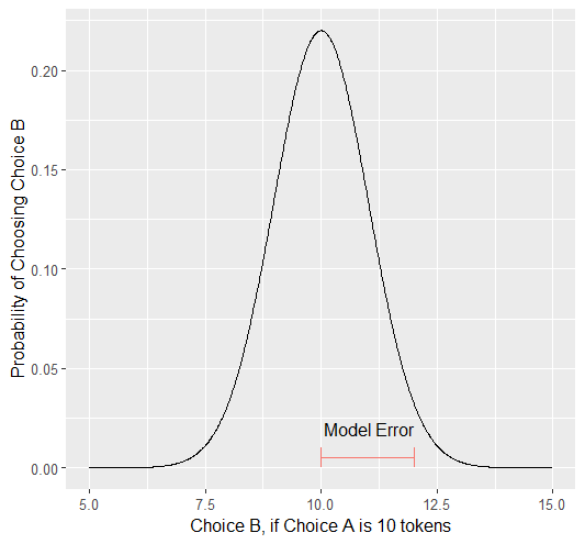
Now, even if we don’t give them the option to return a fraction of a token - meaning we have an interval, rather than a continuous scale - common statistical practice is to treat it as continuous, rather than categorical. In other words, if our model predicts 10 tokens and the Subject actually chooses 12, our error in prediction is better specified as 2 tokens rather than just WRONG. Continuous (or interval) choice tasks aim to elicit Decisions which indicate the the central tendency in a given situation (i.e. the behavior which is mean, median, and mode). Consequently, since 1) our model predicts the central tendency, 2) the distribution around this tendency is normal (an assumption that we’ll check later), and 3) our Free Parameter recovery process is based on the normaility of this distribution (depending on the estimator we use), we don’t need to explicitly capture the probability distribution in our model since it is implicitly captured in how we recover our Free Parameters.
Buttons and Other Categorical Responses
In contrast, consider a binary choice. If we assume that the distribution of these choices is normal, this means something slightly different: using the above picture, let’s imagine a scenario where our Subject has a choice between 10 tokens and 12 tokens. We need to convert this from an outcome distribution to a probability distribution.
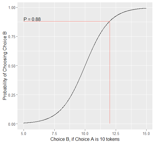
Obviously, this is entirely out of the question - Subjects will disengage after seeing the exact same Trial and having to make the same Decision after 10 or 20 times, much less 100 times. Thus, the only realistic solution is to actually model this probabilistic, noisy Decision process - characterizing how random or noisy this process is. Here, the model will aim to characterize how probable the Subject is to make either possible Decision. In this way, you are essentially hedging your model’s bets which thereby enables your model to overcome sampling error, identifying the central tendency by preventing overcorrection for stochasticity.
Revisiting the above example, if the Subject chooses the 12 tokens, what is our model error?
Predicted Outcome - Observed Outcome = 2 tokens
Wrong Answer = 1 (Binary)
Choice - Probability of Choice = 0.88
Answer
If our model is capturing the noisy, probabilistic nature of decision-making in a binary choice task (which it should, particularly when you don’t have an exorbitant amount of Trials ), our Free Parameters should minimize the probability that our model makes incorrect predictions. Thus, while technically all three could be considered correct, the best answer is ‘C’.
Modeling Sensitivity, Noise, and Bias in Binary Choice Tasks
Now, as we’ll see, we’re going to recover Free Parameters from Decisions by recursively trying different Free Parameters , settling on whichever one minimizes the difference betweeen expected Utility (based on predicted Decisions for a set of Free Parameters ) and observed Utility (based on this same set of Free Parameters and observed Decisions ). Thus far, we’ve talked about Free Parameters which are psychologically interesting, but we must also consider the less interesting parts of decisions when studying binary choices. We will model sensitivity, noise, and bias to ensure that the Free Parameters of interest can be validly and reliably estimated.
Sensitivity
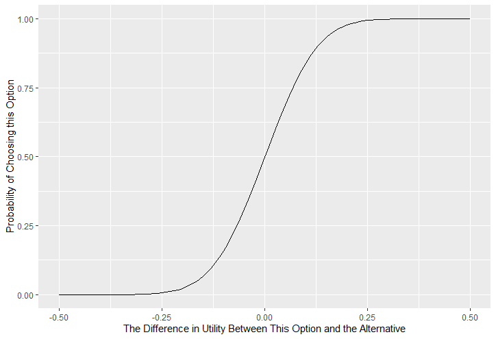
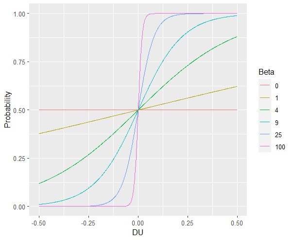
Sensitivity refers to sensitivity to differences in Utility between the two available Choices. Choices which are more different in Utility should be easier to correctly distinguish between. We capture individual differences in sensitivity with the logistic function, where differences in Utility are represented as DU and differences in sensitivity are represented as Beta SF is a scaling function, which can be as high as 100 if the range of DU is 1 or less and as little as 1 if the range of DU is 100 - it depends on your utility function and ranges.
Probability | DU = (1)/(1 + e ** (-Beta * SF * DU))
As you can see, higher values of Beta indicate more sensitivity to differences in Utility
Noise
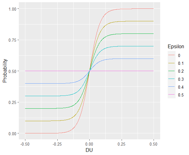
Sometimes, Sensitivity isn’t enough to explain randomness in the Choices people make. Particularly, in the case of these binary choice tasks, it is often the case that doing several hundred trials makes people lose attention - affecting the extent to which their Choices are based on Utility. Thus, this noise can be captured by lessening the extent to which probability is based on DU or Beta and making it closer to 50-50. In other words, (1- Beta) makes the probability of Choices insensitive to DU.
Probability | DU = ((1)/(1 + e ** (-Beta * SF * DU))) * (1 - (1 - Beta)) + (1 - Beta) * 0.5
As you can see, higher values of Epsilon make the probability less based on DU.
Bias
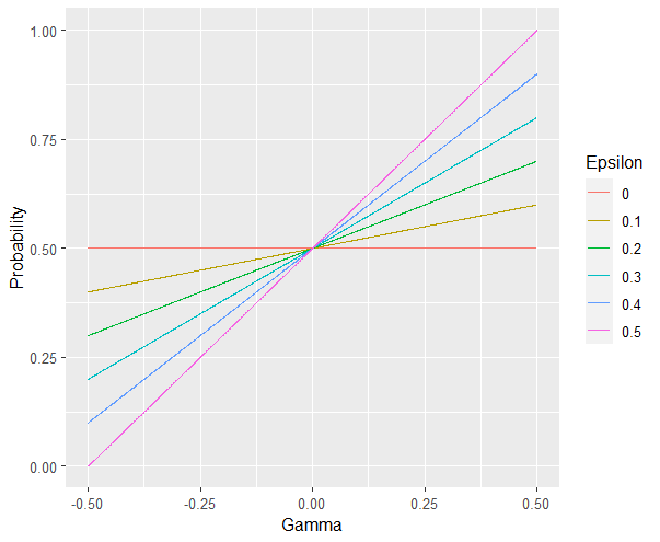
Sometimes, people literally just choose the left or right, or top or bottom more frequently. For now, let’s capture this bias by giving in a new parameter Gamma that modulates the probabilty to reflect this bias. Assume isDirection is a logical (0 is Direction A and 1 is Direction B for instance), we can adjust it to random from -1 to 1. We then multiply (1 - Beta) and Gamma because Gamma should only matter based on the extent to which Choices are insensitive to DU. So, we then combine the factors of (1 - Beta) and Gamma and (2 * isDirection - 1) and add them to the previous probability function.
Probability | DU = ((1)/(1 + e ** (-Beta * SF * DU))) * (1 - (1 - Beta)) + (1 - Beta) * 0.5 + ((1 - Beta) * 0.5 * Gamma * (2 * isDirection - 1))
As you can see, higher values of (1 - Beta) make Gamma the main determinant of the probability.
How to Achieve this Goal
Preallocating, Defining Functions, Defining Trial List, and Defining Parameters
Before you start simulating data, you need to check off a pretty simple list:
Define the Trial List
Define the value of all Independant Variables and all relevant Constants (and all possible Decisions if these do not change from trial-to-trial)
Define Your Functions
Define the value of all Construct Value functions and the Utility function
Define Your Parameters
Define the range and resolution of each of your Free Parameters
Preallocate Model Output
Preallocate the data storage structures for the model-predicted Decisions for each Trial, for each Coordinate (i.e. pair of Free Parameters)
trialList = data.frame(IV = vector(), Constant = vector())

# choices = vector()

utility = function(construct1, construct2, construct3, parameter1, parameter2){
    return(utility)
}

freeParameters = data.frame(parameter1 = vector(),
                            parameter2 = vector())

predictions = data.frame()
trialList = table([], [], 'VariableNames', {'IndependantVariable', 'Constant'});

% choice

function value = construct1(iv, constant, choice)
    value = construct_value;
end

function value = construct2(iv, constant, choice)
    value = construct_value;
end

function value = construct3(iv, constant, choice)
    value = construct_value;
end

function value = utility(construct1, construct2, construct3, parameter1, parameter2)
    value = utility;
end

parameter1range = [];
parameter2range = [];

freeParameters = struct('parameter1', {}, 'parameter2', {}, 'predictions', {});
for i = 1:numel(parameter1range)
    for j = 1:numel(parameter2range)
        freeParameters(i, j).parameter1 = parameter1range(i);
        freeParameters(i, j).parameter2 = parameter2range(j);
        freeParameters(i, j).predictions = zeros(size(triaList, 1), 1);
    end
end
import pandas as pd
import numpy as np

trialList = pd.DataFrame({
    'IndependantVariable': [],
    'Constants': [],
})

# choices = []

def construct1(iv, constant, choice):
    return(construct_value)

def construct2(iv, constant, choice):
    return(construct_value)

def construct3(iv, constant, choice):
    return(construct_value)

def utility(constructs, parameters):
    return(utility)

freeParameters = pd.DataFrame({
    'parameter1': [],
    'parameter2': []
})

predictions = pd.DataFrame()
Define the Free Parameter Loop
We’re going to start our most superior for loop which iterates over unique combinations of Free Parameters.
Each combination of Free Parameters can be thought of as a hypothetical person. In the context of our model, Free Parameters mathematically represent the conceptual dimensions which characterize all of the ways that people can be different in your experimental paradigm. Thus, we are generating predictions about what any given person (i.e. a certain coordinate in our parameter space) would do in our experiment if it is indeed true that our equation aptly represents the data generation process.
So what are we starting with in this loop?
Free Parameters
And what do we want to finish this loop with?
Decisions for all of the Trials in our set.
So what do we need to preallocate before this loop starts?
An output for the predicted Decisions. We already did this above, nice.
Then, what do we need to compute within this loop?
We need to determine what the predicted Decisions for all of the Trials in our set are for those Free Parameters
for (i in 1:length(freeParameters[,1])){
    parameter1 = freeParameters[i,1]
    parameter2 = freeParameters[i,2]

    #Compute Predictions
    predictions[i,] = #To Compute
}
for i = 1:numel(parameter1range)
    for j = 1:numel(parameter2range)
        Parameter1 = freeParameters(i,j).parameter1
        Parameter2 = freeParameters(i,j).parameter2

        %Compute Predictions
        freeParameters(i,j).predictions = %toCompute
    end
end
for i in range(len(freeParameters)):
    Parameter1 = freeParameters[i, 0]
    Parameter2 = freeParameters[i, 1]

    # Compute Predictions
    predictions[i, :] = # To Compute
Define the Trial Loop
Now, we are going to begin answering the Compute Predictions demand placed on us in the Free Parameter Loop. So we’re within the Free Parameter Loop and thus we have our Free Parameter values defined - so let’s say that theoretically we’re adopting the perspective of one hypothetical person. What we want to answer specifically is “What should this hypothetical person do on this particular Trial?”.
So what are we starting with in this loop?
We’re starting with the Independent Variables, Constants, and possible Decisions at the start of each Trial.
We already have Free Parameters defined.
And what do we want to finish this loop with?
The predicted Decision for this Trial.
So what do we need to preallocate before this loop starts?
We need to preallocate a vector for all Decisions for this coordinate pair. However, we already have a preallocated data structure, so for simplicity sake we’ll move that within the Trial loop - defining the model prediction directly on a trial-by-trial basis rather than a coordinate-by-coordinate basis.
Then, what do we need to compute within this loop?
We need to compute the Utility for all possible Decisions in this Trial. Then, we need to save the Decision which results in the greatest Utility.
for (i in 1:length(freeParameters[,1])){
    Parameter1 = freeParameters[i,1]
    Parameter2 = freeParameters[i,2]

    #Just Added
    for (k in 1:length(trialList[,1])){
        IV = trialList[k, 1]
        Constant = trialList[k, 2]
        #Choices = vector() #if not already defined

        # Compute Utility

        predictions[i,k] = # To Compute
    }
}
for i = 1:numel(thetaRange)
    for j = 1:numel(phiRange)
        Parameter1 = freeParameters(i,j).parameter1
        Parameter2 = freeParameters(i,j).parameter2

        %Just Added
        for k = 1:height(trialList(:,1))
            IV = trialList{k,1};
            Constant = trialList{k,2};
            %Choices = []; %if not already defined

            % Compute Utility

            freeParameters(i,j).predictions(k) = %toCompute
        end
    end
end
for i in range(len(freeParameters)):
    Parameter1 = freeParameters[i, 0]
    Parameter2 = freeParameters[i, 1]

    #Just Added
    for k in range(len(trialList)):
        IV = trialList[k, 0]
        Constant = trialList[k, 1]
        #Choices = [] #if not already defined

        # Compute Utility

        predictions[i, k] = # To Compute
Define the Decision Loop
We’re going to start our most inferior for loop which iterates over all possible Decisions.
Here, we’re going to answer the Compute Utility demand placed on us in the Trial loop.
So what are we starting with in this loop?
We’re starting with one of the possible Decisions at the start of each loop.
We already have Independent Variables, Constants, and possible Decisions defined at the start of the Trial loop and
Free Parameters defined at the start of the Free Parameter loop.
And what do we want to finish this loop with?
The Utility which would be derived for all Decisions on this Trial.
So what do we need to preallocate before this loop starts?
A vector for Utility which has the same length as all possible Decisions.
Also, let’s remember that it’s possible that multiple Decisions will maximize utility. Therefore, let’s make sure that our script doesn’t error by potentially outputting multiple Decisions predictions - we’ll randomly select between whichever maximizes utility. Let’s also output a vector which keeps track of the number of Trials where multiple Decisions maximize Utility (i.e. our model makes non-specific predictions) for each pair of Free Parameters. A few of Trials for a few Free Parameters is acceptable, but let’s just keep an eye on it.
Then, what do we need to compute within this loop?
Nothing, this is the smallest loop. We’re ready to get our answer.
non_specific = rep(0, length(freeParameters[,1])) # Just Added This Line

for (i in 1:length(freeParameters[,1])){
    Parameter1 = freeParameters[i,1]
    Parameter2 = freeParameters[i,2]
    for (k in 1:length(trialList[,1])){
        IV = trialList[k, 1]
        Constant = trialList[k, 2]
        #Choices = vector() #if not already defined

        # Just Added
        Utility = vector('numeric', length(Choices))
        for (n in 1:length(Choices)){
            Utility[n] = utility(parameter1 = Parameter1,
                                parameter2 = Parameter2,
                                construct1 = construct1(IV, Constant, Choices[n]),
                                construct2 = construct2(IV, Constant, Choices[n]),
                                construct3 = construct3(IV, Constant, Choices[n]))
        }
        correct_choice = which(Utility == max(Utility))
        if (length(correct_choice) > 1){
            correct_choice = correct_choice[sample(correct_choice, 1)]
            non_specific[i] =+ 1
        }
        predictions[i,k] = Choices[correct_choice]
    }
}
freeParameters = struct('theta', {}, 'phi', {}, 'predictions', {}, 'non_specific', {}); %Just Changed This Line

for i = 1:numel(thetaRange)
    for j = 1:numel(phiRange)
        Parameter1 = freeParameters(i,j).parameter1
        Parameter2 = freeParameters(i,j).parameter2

        %Just Added
        for k = 1:height(trialList(:,1))
            IV = trialList{k,1};
            Constant = trialList{k,2};
            %Choices = []; %if not already defined

            % Just Added
            Utility = zeros(size(Choices));
            for n = 1:height(Choices(:,1))
                Utility(n) = utility(parameter1 = Parameter1,
                                    parameter2 = Parameter2,
                                    construct1 = construct1(IV, Constant, Choices[n]),
                                    construct2 = construct2(IV, Constant, Choices[n]),
                                    construct3 = construct3(IV, Constant, Choices[n]))
            end
            correct_choice = find(Utility == max(Utility));
            if numel(correct_choice) > 1
                correct_choice = correct_choice(randi(numel(correct_choice)));
                freeParameters(i,j).non_specific(k) = freeParameters(i,j).non_specific(k) + 1;
            end
            freeParameters(i,j).predictions(k) = Choices(correct_choice)
        end
    end
end
non_specific = [0] * len(freeParameters) # Just Added this Line

for i in range(len(freeParameters)):
    Parameter1 = freeParameters[i, 0]
    Parameter2 = freeParameters[i, 1]

    for k in range(len(trialList)):
        IV = trialList[k, 0]
        Constant = trialList[k, 1]
        #Choices = [] #if not already defined

        #Just Added
        Utility = [0] * len(Choices)
        for n in range(len(Choices)):
            Utility[n] = utility(parameter1 = Parameter1,
                                parameter2 = Parameter2,
                                construct1 = construct1(IV, Constant, Choices[n]),
                                construct2 = construct2(IV, Constant, Choices[n]),
                                construct3 = construct3(IV, Constant, Choices[n]))

        correct_choice = [idx for idx, val in enumerate(Utility) if val == max(Utility)]
        if len(correct_choice) > 1:
            correct_choice = random.sample(correct_choice, 1)
            non_specific[i] += 1

        predictions[i, k] = Choices[correct_choice[0]]
Tutorials
Tutorial 1 - van Baar, Chang, & Sanfey, 2019
Preallocating, Defining Functions, Defining Trial List, and Defining Parameters
#Construct Value Formulations Above this
trialList = data.frame(Investment = rep(seq(1, 10, 1), times = 6),
                       Multiplier = rep(c(2, 4, 6), each = 20),
                       Believed_Multiplier = rep(4, 60),
                       Endowment = rep(10, 60))

utility = function(theta, phi, guilt, inequity, payout){
    return(theta*payout - (1-theta)*min(guilt + phi, inequity - phi))
}

freeParameters = data.frame(theta = rep(seq(0, 0.5, 0.005), each = 101),
                            phi = rep(seq(-0.1, 0.1, 0.002), times = 101))

predictions = data.frame()
trialList = table(repelem(1:10, 6)', repmat([2; 4; 6], 20, 1), repmat(4, 60, 1), repmat(10, 60, 1), 'VariableNames', {'Investment', 'Multiplier', 'Believed_Multiplier', 'Endowment'});

function value = payout_maximization(investment, multiplier, returned)
    value = ((investment * multiplier) - returned) / (investment * multiplier);
end

function value = inequity(investment, multiplier, returned, endowment)
    value = ((investment * multiplier - returned)/(investment * multiplier + endowment - investment))^2;
end

function value = guilt(investment, believed_multiplier, returned, multiplier)
    value = ((investment * believed_multiplier)/2 - returned) / (investment * multiplier);
end

function value = utility(theta, phi, guilt, inequity, payout)
    value = (theta*payout - (1-theta)*min(guilt + phi, inequity - phi));
end

thetaRange = 0:0.005:0.5;
phiRange = -0.1:0.002:0.1;

freeParameters = struct('theta', {}, 'phi', {}, 'predictions', {});
for i = 1:numel(thetaRange)
    for j = 1:numel(phiRange)
        freeParameters(i, j).theta = thetaRange(i);
        freeParameters(i, j).phi = phiRange(j);
        freeParameters(i, j).predictions = zeros(80, 1); % Empty vector of length 80
    end
end
import pandas as pd
import numpy as np

Investment = np.repeat(np.arange(1, 11), repeats=6)
Multiplier = np.repeat([2, 4, 6], repeats=20)
Believed_Multiplier = np.repeat(4, 60)
Endowment = np.repeat(10, 60)

trialList = pd.DataFrame({
    'Investment': Investment,
    'Multiplier': Multiplier,
    'Believed_Multiplier': Believed_Multiplier,
    'Endowment': Endowment
})

def utility(theta, phi, guilt, inequity, payout):
    return(theta*payout - (1-theta)*min(guilt + phi, inequity - phi))

theta = np.repeat(np.arange(0, 0.505, 0.005), repeats=101)
phi = np.tile(np.arange(-0.1, 0.102, 0.002), 101)

freeParameters = pd.DataFrame({
    'theta': theta,
    'phi': phi
})

predictions = pd.DataFrame()
Define the Free Parameter Loop
for (i in 1:length(freeParameters[,1])){
    Theta = freeParameters[i,1]
    Phi = freeParameters[i,2]

    #Compute Predictions
    predictions[i,] = #To Compute
}
for i = 1:numel(thetaRange)
    for j = 1:numel(phiRange)
        Theta = freeParameters(i,j).theta
        Phi = freeParameters(i,j).phi

        %Compute Predictions
        freeParameters(i,j).predictions = %toCompute
    end
end
for i in range(len(freeParameters)):
    Theta = freeParameters[i, 0]
    Phi = freeParameters[i, 1]

    # Compute Predictions
    predictions[i, :] = # To Compute
Define the Trial Loop
for (i in 1:length(freeParameters[,1])){
    Theta = freeParameters[i,1]
    Phi = freeParameters[i,2]

    #Just Added
    for (k in 1:length(trialList[,1])){
        I = trialList[k, 1]
        M = trialList[k, 2]
        B = trialList[k, 3]
        E = trialList[k, 4]
        Choices = seq(0, (I * M), 1)

        # Compute Utility

        predictions[i,k] = # To Compute
    }
}
for i = 1:numel(thetaRange)
    for j = 1:numel(phiRange)
        Theta = freeParameters(i,j).theta
        Phi = freeParameters(i,j).phi

    %Just Added
        for k = 1:height(trialList(:,1))
            I = trialList{k,1};
            M = trialList{k,2};
            B = trialList{k,3};
            E = trialList{k,4};
            Choices = 0:1:(I*M);

            % Compute Utility

            freeParameters(i,j).predictions(k) = %toCompute
        end
    end
end
for i in range(len(freeParameters)):
    Theta = freeParameters[i, 0]
    Phi = freeParameters[i, 1]

    #Just Added
    for k in range(len(trialList)):
        I = trialList[k, 0]
        M = trialList[k, 1]
        B = trialList[k, 2]
        E = trialList[k, 3]
        Choices = list(range(0, I * M + 1, 1))

        # Compute Utility

        predictions[i, k] = # To Compute
Define the Decision Loop
non_specific = rep(0, length(freeParameters[,1])) # Just Added This Line

for (i in 1:length(freeParameters[,1])){
    Theta = freeParameters[i,1]
    Phi = freeParameters[i,2]

    for (k in 1:length(trialList[,1])){
        I = trialList[k, 1]
        M = trialList[k, 2]
        B = trialList[k, 3]
        E = trialList[k, 4]
        Choices = seq(0, (I * M), 1)

        # Just Added
        Utility = vector('numeric', length(Choices))
        for (n in 1:length(Choices)){
            Utility[n] = utility(theta = Theta,
                                phi = Phi,
                                guilt = guilt(I, B, Choices[n], M),
                                inequity = inequity(I, M, Choices[n], E),
                                payout = payout_maximization(I, M, Choices[n]))
        }
        correct_choice = which(Utility == max(Utility))
        if (length(correct_choice) > 1){
            correct_choice = correct_choice[sample(1:length(correct_choice), 1)]
            non_specific[i] =+ 1
        }
        predictions[i,k] = Choices[correct_choice]
    }
}
freeParameters = struct('theta', {}, 'phi', {}, 'predictions', {}, 'non_specific', {}); %Just Added this Line

for i = 1:numel(thetaRange)
    for j = 1:numel(phiRange)
        Theta = freeParameters(i,j).theta
        Phi = freeParameters(i,j).phi

        for k = 1:height(trialList(:,1))
            I = trialList{k,1};
            M = trialList{k,2};
            B = trialList{k,3};
            E = trialList{k,4};
            Choices = 0:1:(I*M);

            %Just Added
            Utility = zeros(size(Choices));
            for n = 1:height(Choices(:,1))
                Utility(n) = utility(theta = Theta,
                                     phi = Phi,
                                     guilt = guilt(I, B, Choices(n), M),
                                     inequity = inequity(I, M, Choices(n), E),
                                     payout = payout_maximization(I, M, Choices(n)))
            end
            correct_choice = find(Utility == max(Utility));
            if numel(correct_choice) > 1
                correct_choice = correct_choice(randi(numel([1:height(correct_choice)])));
                freeParameters(i,j).non_specific(k) = freeParameters(i,j).non_specific(k) + 1;
            end
            freeParameters(i,j).predictions(k) = Choices(correct_choice)
        end
    end
end
import random

non_specific = [0] * len(freeParameters) # Just Added this Line

for i in range(len(freeParameters)):
    Theta = freeParameters[i, 0]
    Phi = freeParameters[i, 1]

    for k in range(len(trialList)):
        I = trialList[k, 0]
        M = trialList[k, 1]
        B = trialList[k, 2]
        E = trialList[k, 3]
        Choices = list(range(0, I * M + 1, 1))

        #Just Added
        Utility = [0] * len(Choices)
        for n in range(len(Choices)):
            Utility[n] = utility(theta=Theta,
                                phi=Phi,
                                guilt=guilt(I, B, Choices[n], M),
                                inequity=inequity(I, M, Choices[n], E),
                                payout=payout_maximization(I, M, Choices[n]))

        correct_choice = [idx for idx, val in enumerate(Utility) if val == max(Utility)]
        if len(correct_choice) > 1:
            correct_choice = random.sample(range(len(correct_choice)), 1)
            non_specific[i] += 1

        predictions[i, k] = Choices[correct_choice[0]]
Tutorial 2 - Galvan & Sanfey, 2024
Preallocating, Defining Functions, Defining Trial List, and Defining Parameters
#first, create a noisy resource distribution that has gini between 0.3 and 0.4 where the maximum benefit or loss is approximately going to be 10 tokens
shares = seq(0.05,0.95, 0.1)**1.25
df = data.frame()
for (k in 1:10){
    df[1:20, k] = rnorm(20, mean=shares[k], sd=0.01*sum(shares))
    df[which(df[,k] < 0),] = 0
}

#second, convert to a rounded percent
for (k in 1:length(df[,1])) {
    df[k,1:10] = round((df[k,1:10]/sum(df[k,1:10]))*100)
}

#third, ensure that there are exactly 100 tokens on each trial
for (k in 1:length(df[,1])) {
    if (sum(df[k,1:10]) < 100){
        for (j in 1:(100-sum(df[k,1:10]))){
        i = sample(1:10, 1)
        df[k, i] = df[k, i] + 1
        }
    }
    if (sum(df[k,1:10]) > 100){
        for (j in 1:(sum(df[k,1:10]) - 100)){
        i = sample(which(df[k,1:10] > 0), 1)
        df[k, i] = df[k, i] - 1
        }
    }
}

trialList = data.frame()

#fourth, ensure that our subject is in each decile the same number of times
for (k in 1:length(df[,1])){
    i = round((k/2)+0.05) #because this function rounds down on even numbers and up on odd numbers
    trialList[k, 1] = df[k, i]
    intermediate = df[k, -i]
    trialList[k, 2:10] = intermediate[1,sample(9)] #to insure that other players on screen are not all
}

#trialList above
choices = seq(0, 1, 0.1) #tax rate

utility = function(theta, phi, Equity, Equality, Payout){
    return((theta * Payout) + ((1 - theta) * ((phi * Equality) + ((1 - phi) * Equity))))
}

freeParameters = data.frame(theta = seq(0, 1, 0.01),
                            phi = seq(0, 1, 0.01))

predictions = data.frame()
% First, create a noisy resource distribution
shares = (0.05:0.1:0.95).^1.25;
df = zeros(20, 10);

for k = 1:10
    df(:, k) = normrnd(shares(k), 0.01 * sum(shares), [20, 1]);
    df(df(:, k) < 0, k) = 0;
end

% Second, convert to a rounded percent
for k = 1:length(df(:, 1))
    df(k, 1:10) = round((df(k, 1:10) / sum(df(k, 1:10))) * 100);
end

% Third, ensure that there are exactly 100 tokens on each trial
for k = 1:length(df(:, 1))
    if sum(df(k, 1:10)) < 100
        for j = 1:(100 - sum(df(k, 1:10)))
            i = randi(10);
            df(k, i) = df(k, i) + 1;
        end
    elseif sum(df(k, 1:10)) > 100
        for j = 1:(sum(df(k, 1:10)) - 100)
            i = find(df(k, 1:10) > 0);
            i = i(randi(length(i)));
            df(k, i) = df(k, i) - 1;
        end
    end
end

% Fourth, ensure that our subject is in each decile the same number of times
trialList = zeros(length(df(:, 1)), 10);

for k = 1:length(df(:, 1))
    i = round((k / 2) + 0.05);
    trialList(k, 1) = df(k, i);
    intermediate = df(k, [1:i-1, i+1:end]);
    trialList(k, 2:10) = intermediate(1, randi(9));
end

% choices above
choices = 0:0.1:1; % tax rate

% Define utility function
utility = @(theta, phi, Equity, Equality, Payout) (theta * Payout) + ((1 - theta) * ((phi * Equality) + ((1 - phi) * Equity)));

% Define free parameters as a structure
freeParameters = struct('theta', linspace(0, 1, 101), 'phi', linspace(0, 1, 101));

% Pre-allocate predictions as a structure
predictions = struct('result', cell(101, 101));

% Loop over freeParameters
for i = 1:length(freeParameters.theta)
    for j = 1:length(freeParameters.phi)
        % Access current parameter values
        theta_val = freeParameters.theta(i);
        phi_val = freeParameters.phi(j);

        % Your utility function call here using theta_val and phi_val

        % Store the result in predictions structure
        predictions(i, j).result = result;
    end
end
import numpy as np

# First, create a noisy resource distribution
shares = (np.arange(0.05, 1, 0.1)**1.25)
df = np.zeros((20, 10))

for k in range(10):
    df[:, k] = np.random.normal(shares[k], 0.01 * np.sum(shares), 20)
    df[df[:, k] < 0, k] = 0

# Second, convert to a rounded percent
for k in range(len(df[:, 0])):
    df[k, 0:10] = np.round((df[k, 0:10] / np.sum(df[k, 0:10])) * 100)

# Third, ensure that there are exactly 100 tokens on each trial
for k in range(len(df[:, 0])):
    if np.sum(df[k, 0:10]) < 100:
        for j in range(100 - int(np.sum(df[k, 0:10]))):
            i = np.random.randint(10)
            df[k, i] = df[k, i] + 1
    elif np.sum(df[k, 0:10]) > 100:
        for j in range(int(np.sum(df[k, 0:10])) - 100):
            i = np.random.choice(np.where(df[k, 0:10] > 0)[0])
            df[k, i] = df[k, i] - 1

# Fourth, ensure that our subject is in each decile the same number of times
trialList = np.zeros((len(df[:, 0]), 10))

for k in range(len(df[:, 0])):
    i = round((k / 2) + 0.05)
    trialList[k, 0] = df[k, i]
    intermediate = np.delete(df[k, :], i)
    trialList[k, 1:10] = np.random.choice(intermediate, 9)

# choices above
choices = np.arange(0, 1.1, 0.1)  # tax rate

# Define utility function
def utility(theta, phi, Equity, Equality, Payout):
    return (theta * Payout) + ((1 - theta) * ((phi * Equality) + ((1 - phi) * Equity)))

# Define free parameters
theta_values = np.arange(0, 1.01, 0.01)
phi_values = np.arange(0, 1.01, 0.01)
freeParameters = np.array(np.meshgrid(theta_values, phi_values)).T.reshape(-1, 2)
Define the Free Parameter Loop
non_specific = rep(0, length(freeParameters[,1])) # Just Added This Line

for (i in 1:length(freeParameters[,1])){
    Theta = freeParameters[i,1]
    Phi = freeParameters[i,2]

    #Define Trials
}
non_specific = zeros(1, numel(freeParameters.theta));

for i = 1:numel(freeParameters.theta)
    Theta = freeParameters.theta(i);
    Phi = freeParameters.phi(i);

    % Define Trials
end
non_specific = np.zeros(len(freeParameters['theta']))

for i in range(len(freeParameters['theta'])):
    Theta = freeParameters['theta'][i]
    Phi = freeParameters['phi'][i]

    non_specific[i] = some_result  # Replace some_result with your actual result
Define the Trial Loop
non_specific = rep(0, length(freeParameters[,1])) # Just Added This Line

for (i in 1:length(freeParameters[,1])){
    Theta = freeParameters[i,1]
    Phi = freeParameters[i,2]

    #Just Added
    for (k in 1:length(trialList[,1])){

        #Determine Predicted Decisions
    }
}
non_specific = zeros(1, numel(freeParameters.theta));

for i = 1:numel(freeParameters.theta)
    Theta = freeParameters.theta(i);
    Phi = freeParameters.phi(i);

    for k = 1:numel(trialList(:, 1))
        % Determine Predicted Decisions
    end
end
non_specific = np.zeros(len(freeParameters['theta']))

for i in range(len(freeParameters['theta'])):
    Theta = freeParameters['theta'][i]
    Phi = freeParameters['phi'][i]

    for k in range(len(trialList[:, 0])):
        # Determine Predicted Decisions
Define the Decision Loop
non_specific = rep(0, length(freeParameters[,1])) # Just Added This Line

for (i in 1:length(freeParameters[,1])){
    Theta = freeParameters[i,1]
    Phi = freeParameters[i,2]
    for (k in 1:length(trialList[,1])){

        # Just Added
        Utility = vector('numeric', length(choices))
        for (n in 1:length(choices)){
            Utility[n] = utility(theta = Theta,
                                 phi = Phi,
                                 Equity = equity(new_value(trialList[k, 1:10], choices[n]), trialList[k, 1:10], choices[n]),
                                 Equality = equality(new_value(trialList[k, 1:10], choices[n]), trialList[k, 1:10], choices[n]),
                                 Payout = payout(new_value(trialList[k, 1], choices[n]), trialList[k, 1], choices[n]))
        }
        correct_choice = which(Utility == max(Utility))
        if (length(correct_choice) > 1){
            correct_choice = correct_choice[sample(correct_choice, 1)]
            non_specific[i] =+ 1
        }
        predictions[i,k] = Choices[correct_choice]
    }
}
non_specific = zeros(1, numel(freeParameters.theta));

for i = 1:numel(freeParameters.theta)
    Theta = freeParameters.theta(i);
    Phi = freeParameters.phi(i);

    for k = 1:numel(trialList(:, 1))
        % Just Added
        Utility = zeros(size(choices));

        for n = 1:length(choices)
            Equity = equity(new_value(trialList(k, 1:10), choices(n)), trialList(k, 1:10), choices(n));
            Equality = equality(new_value(trialList(k, 1:10), choices(n)), trialList(k, 1:10), choices(n));
            Payout = payout(new_value(trialList(k, 1), choices(n)), trialList(k, 1), choices(n));

            Utility(n) = utility(Theta, Phi, Equity, Equality, Payout);
        end

        [~, correct_choice] = max(Utility);
        if numel(correct_choice) > 1
            correct_choice = correct_choice(randi(numel(correct_choice), 1));
            non_specific(i) = non_specific(i) + 1;
        end

        predictions(i, k) = choices(correct_choice);
    end
end
non_specific = np.zeros(len(freeParameters['theta']))

for i in range(len(freeParameters['theta'])):
    Theta = freeParameters['theta'][i]
    Phi = freeParameters['phi'][i]

    for k in range(len(trialList[:, 0])):
        # Just Added
        Utility = np.zeros(len(choices))

        for n in range(len(choices)):
            Equity = equity(new_value(trialList[k, 0:10], choices[n]), trialList[k, 0:10], choices[n])
            Equality = equality(new_value(trialList[k, 0:10], choices[n]), trialList[k, 0:10], choices[n])
            Payout = payout(new_value(trialList[k, 0], choices[n]), trialList[k, 0], choices[n])

            Utility[n] = utility(Theta, Phi, Equity, Equality, Payout)

        correct_choice = np.argmax(Utility)
        if np.sum(Utility == Utility[correct_choice]) > 1:
            correct_choice = np.random.choice(np.where(Utility == np.max(Utility))[0])
            non_specific[i] += 1

        predictions[i, k] = choices[correct_choice]
Tutorial 3 - Crockett et al., 2014
Preallocating, Defining Functions, Defining Trial List, and Defining Parameters
trialList = data.frame(Default = rep(c(1, 2), each = 100),
                       MoneyA = 10,
                       MoneyB = rep(rep(seq(11, 20), each = 10), times = 2),
                       ShocksA = rep(rep(seq(0, 9), times = 10), times = 2),
                       ShocksB = 10)

utility = function(Payout, Harm, kappa, lambda){
    if (Payout < 0) {LM = lambda} else {LM = 1}
    if (Harm > 0) {LS = lambda} else {LS = 1}
    return((Payout * kappa * LM) - (Harm * (1 - kappa) * LS))
}

freeParameters = data.frame(kappa = rep(seq(0, 1, 0.1), 11), #ranging from 0 to 1, the inverse of kappa has the same range as kappa
                            lambda = rep(seq(1, 3, 0.2), 11), #loss aversion is 2.25 according to CPT, 1 is no loss aversion
                            gamma = sample(seq(0, 2, 0.01), 121), #completely random to low stochasticity
                            epsilon = 0) #no additional, non-task related noise
predictions = data.frame()
Define the Free Parameter Loop
for (i in 1:length(freeParameters[,1])){
    Kappa = freeParameters[i,1]
    Lambda = freeParameters[i,2]

    #Define Trial Loop

}
Define the Trial Loop
for (i in 1:length(freeParameters[,1])){
    Kappa = freeParameters[i,1]
    Lambda = freeParameters[i,2]

    #Just Added
    for (k in 1:length(trialList[,1])){
        shocksThis = c(trialList$ShocksA[k], trialList$ShocksB[k])[trialList$Default[k]]
        shocksAlternative = c(trialList$ShocksB[k], trialList$ShocksA[k])[trialList$Default[k]]
        moneyThis = c(trialList$MoneyA[k], trialList$MoneyB[k])[trialList$Default[k]]
        moneyAlternative = c(trialList$MoneyB[k], trialList$MoneyA[k])[trialList$Default[k]]

        # Determine predictions

    }
}
Determine the Predicted Decision
for (i in 1:length(freeParameters[,1])){
    Kappa = freeParameters[i,1]
    Beta = freeParameters[i,2]
    Epsilon = freeParameters[i,3]
    Gamma = freeParameters[i,4]
    for (k in 1:length(trialList[,1])){
        shocksMore = trialList$ShocksA[k]
        shocksLess = trialList$ShocksB[k]
        moneyMore = trialList$MoneyA[k]
        moneyLess = trialList$MoneyB[k]

        # Just Added
        Utility = utility(Harm = harm(shocksMore, shocksLess),
                        Payout = payout(moneyMore, moneyLess),
                        kappa = Kappa)
        predictions[i,k] = as.numeric(round(probability(Beta, Epsilon, Gamma, Utility, trialList$Left[k]) * 1000)> sample(1000,1))
    }
}
Tutorial 4 - Li et al., 2014
Note
In this final tutorial, we will shift our programming away from writing repetitive code to instead use functions. One of the most repetitive things we do when modeling is generating predictions. In the function generatePredictions, we will generate predictions based on the Free Parameters and Trial Set.
Preallocating, Defining Functions, Defining Trial List, and Defining Parameters
trialList = data.frame(a0 = sample(10:20, 100, replace = T))
trialList$b0 = 20 - trialList$a0
for (i in 1:nrow(trialList)){
    trialList$a1 = sample(5:trialList$a0[i], 100, replace = T)
}
trialList$b1 = 20 - trialList$a1

for (i in 1:nrow(trialList)){
    trialList$a2 = sample(5:trialList$a0[i], 100, replace = T)
    trialList$a2[which(trialList$a2 == trialList$a1)] = 10
}
trialList$b2 = 20 - trialList$a2
trialList = rbind(trialList, trialList[,c(2,1,4,3,6,5)])

utility = function(pars, IVs){
    IVS = as.numeric(IVs)
    a0 = IVs[1]; b0 = IVs[2]; a1 = IVs[3]; b1 = IVs[4]; a2 = IVs[5]; b2 = IVs[6]
    alpha = pars[1]; delta = pars[2]; rho = pars[3]
    inequality = inequality(a1, b1, a2, b2)
    harm = harm(a0, b0, a1, b1, a2, b2)
    rank = rankReverse(a0, b0, a1, b1, a2, b2)
    return((alpha * inequality) - (delta * harm) - (rho * rank))
}

probability = function(pars, utilitydiff){
    beta = pars[length(pars)-2]; epsilon = pars[length(pars)-1]; gamma = pars[length(pars)]
    prob = 1 / (1 + exp(-(beta * utilitydiff)))
    prob = prob * (1 - 2 * epsilon) + epsilon + gamma * (2 * epsilon)
    return(prob)
}

freeParameters = data.frame(alpha = rep(rep(seq(0, 1.5, 0.5), times = 16), each = 6) + sample(seq(0, 0.5, 0.001), 6*64, replace = T), #ranging from 0 to 2
                            delta = rep(rep(rep(seq(0, 1.5, 0.5), times = 4), each = 4), each = 6) + sample(seq(0, 0.5, 0.001), 6*64, replace = T), #ranging from 0 to 2
                            rho = rep(rep(seq(0, 1.5, 0.5), each = 16), each = 6) + sample(seq(0, 0.5, 0.001), 6*64, replace = T), #ranging from 0 to 2
                            beta = sample(seq(0,10), 6*64, replace = T), # stochasticity
                            epsilon = rep(seq(0, 0.5, 0.1), times = 64), # noise
                            gamma = sample(seq(-0.5, 0.4, 0.1), 64*6, replace = T) + sample(seq(0, 0.1, 0.001), 64*6, replace = T)) # bias

predictions = data.frame()

generatePredictions = function(parameters, df){
    pred = vector('numeric', nrow(df))
    for (i in 1:nrow(df)){
        thisTrialIVs = as.numeric(df[i, ])
        utilityDiff = utility(parameters, thisTrialIVs)
        pred[i] = max(min(probability(parameters, utilityDiff), 0.9999999999), 0.00000000001)
    }
    return(pred)
}
Define the Free Parameter Loop
for (i in 1:nrow(freeParameters)){
    pars = freeParameters[i, ]
    predictions[i, 1:nrow(trialList)] = as.numeric(round(generatePredictions(pars, trialList) * 1000)> sample(1000,1))
}