Grouping

Lesson

Elijah Galvan

September 1, 2023

13 min read

Goal During this Stage

To examine our model predictions in an efficient way and to potentially generate theoretical, sampling invariant, theoretically valid a priori groupings. Essentially, this a valid, unbiased way to classify subjects’ behavior in your task without making any arbitrary assertions about who falls into which group.

How to Achieve this Goal

Note

This section will differ from the previous sections: rather than provide conceptual examples about how to implement it, we’ll primarily talk about the reasons to use this approach and what it can be used for. The implementation examples will be in reference to the first tutorial.

Choosing an Approach to Grouping

Canonically, there have been 2 approaches to grouping: clustering and binning.

Binning is simply the researcher asserting that it is the case that groups 1 and 2 are differentiable on X or Y: the grouping is only as valid as the researcher’s reasoning. Further, this approach is theoretically only valid when specified a priori (in a preregistration).

On the other hand, Clustering is an empirical, data-driven approach which provides post-hoc explanations. Essentially, whichever Clustering Algorithm you use searches for the best solution to the problem you offer it. Thus, the groups are determined by the observed data and can obviously be biased therein.

Here, we clearly don’t have any real data: we want to cluster the simulated model predictions. This is the most ideal situation: since we can simulate as much data as we want and therefore exhaustively represent the variance in expected behavior. Here, we also group based on the model predictions (i.e. our hypotheses) - which means that our clustered groupings are a logical extension of our psychological theory in the context of our Experimental Paradigm and Trial Set. This enables us to overcome the limitations of both clustering (post-hoc, sampling dependency, atheoretical) and binning (arbitrariness, overreliance on reasoning, etc.).

However, the validity of a priori clustering requires that our model be highly generalizable: all Constructs must have the same value on the same Trial for each subject and there are no Free Parameters in your model which do not translate to psychologically meaningful differences.. So, for instance, this might preclude using binary choice tasks which often require Free Parameters to model response bias parameters (preference for left-versus-right) and inverse heat parameters (probability of behaving preference-congruent) for example. It also requires that all Constructs are directly computed from Experimental Variables and not self-report measures for instance. In this study, the experimenters asked what the participant thought the Investor expected for all trials: although this would be a theoretically superior way to mathematically calculate Guilt, using the a priori clustering to group subjects would be conceptually problematic. In these cases, it is always good to make sure that the generalized Constructs is highly correlated with the questionnaire measure and that using either value leads to the same behavioral conclusions - not just taking for granted that these are distinctions without differences.

Choosing a Clustering Algorithm

Clustering Algorithms are generally used to determine 1) how many groups are in a data set and 2) the group that people belong to in a data set. They do this by taking one observation of multiple variables (columns) for many people (rows). As an input Hierarchical Agglomerative Clustering (HAC), which is what we will be using, takes a distance matrix. A distance matrix is a square matrix with as many rows and columns as the number of rows in our data set. Every cell below the diagonal (i.e. the second-last row of the first column, the third-last row of the second column, etc.) represents a distance. Here, distance is often Euclidean meaning it is just an extension of Pythagorean Theorem - it equals the sum of all squared differences between the values in each column. The position of the cell is also meaningful: for instance, the cell in the first row and the second column represents the total distance between Subject 1 and Subject 2 for instance.

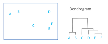
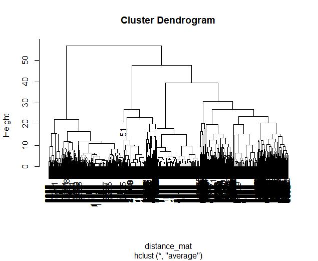
HAC essentially tries to figure out what the most parsimonious grouping is for each possible number of groups, starting with 2 groups and finishing with the maximum number of groups (i.e. the number of rows meaning everyone is in their own group). It visualizes this parsimony in the form of a dendrogram - a type of tree graph. Reading dendrograms is simple, but for some people it is not very intuitive. You determine the number of groups in a data set by cutting the tree. You determine where to cut the tree on the horizontal where there is the longest vertical space without any branching. To develop an intuition about these things, see the image below which we would cut into 2 groups - group 1 with [A, B] and group 2 with [C, D, E, F].

Note

There are many different clustering algorithms out there, but I’ll only be talking about HAC because it is basic, I’m agnostic about clustering algorithms, and I’m familiar with it. You might have a strong opinion or motivation - in principle, any clustering algorithm can be applied and your needs and knowledge might dictate that others are preferable and that’s perfectly valid.

Informing a Change in the of Trial Set

Our Trial Set is designed to elicit maximally different behavioral patterns between groups of people who have different psychological preferences. Some rules of thumb here are as follows:

1. Offer as many choice options as is possible, within reason

2. Make sure the number of trials in each condition of interest are equal

Here, HAC especially can offer insight about if you have accomplished these two aims. Let’s take a look at some minor mistakes that were made in this study.

Limited Choice Options and Asymetric Trial Set

In the paper, the Choice Options were in increments of 1 token or 10% of the slider range (whichever was greatest, to increase the speed of movement on the slider and the trial distribution was not 10 trials per multiplier condition (with Investment ranging fro 1 to 10). For the exact trial distribution you can see the file trialSet.csv in the folder that you downloaded with the actual data.

Note

The authors also conducted a behavioral follow-up to validate a different clustering which they applied in the paper.

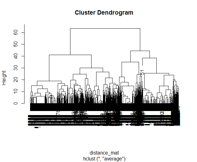
Using HAC on these simulations leads to the following dendrogram which favors a 2 group solution and the following model space which is less in line with our expected outcome of either a 3 or 4 cluster solution as specified in our hypotheses.

Dendgrogram for the fMRI Experiment

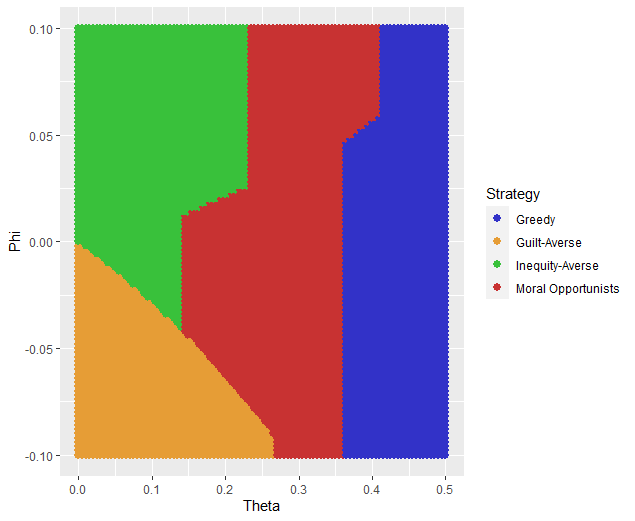
It also leads to the following grouping for a 4 cluster solution which is not well aligned with the parameter space that we sketched out earlier.

Model Space for the fMRI Experiment

Having the Choice Options always Specified in Increments of 1 Token leads to the following with the same Trial Set

Asymetric Trial Set

Dendgrogram

Model Space

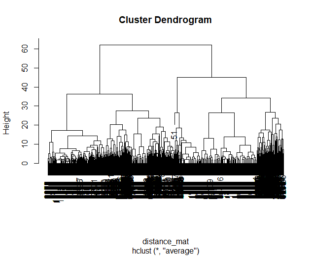
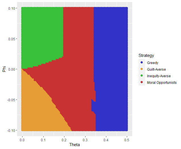
Fixing both of these problems - which the authors did in the behavioral follow-up also reported in the paper - results in the following.

The Ideal Trial Set

Dendgrogram

Model Space

Tutorials

Tutorial 1 - van Baar, Chang, & Sanfey, 2019

Choosing an Approach to Grouping

Our four choices are: no grouping, binning, a priori clustering, or post-hoc clustering. Since we want to study people based on the strategy that they use to make decisions and our model is not using noise parameters, let’s group. The reason we don’t have to include noise parameters is because we are offering several choices per trial, so a priori clustering is on the table. Binning isn’t appropriate here because we’re looking for 4 strategies and the cutoffs between these strategies are kind of fuzzy - we don’t want to arbitrarily assign boundaries between strategies if we can avoid it. Post-hoc clustering isn’t preferable when we can group a priori, so let’s do that.

Cluster Your Data Using HAC

Plain English

We need to compute a distance matrix which will require a table or data frame object which contains the model predictions. Then we will use an HAC algorithm to cluster the data. After, we will determine how many groups we should have and we will cut the tree into that many groups - assigning row identities to whichever group the clustering algorithm says that they belong to.

R

distance_mat = dist(predictions, method = 'euclidean')
set.seed(240)
hierarchical = hclust(distance_mat, method = 'average')
plot(hierarchical)
fit = cutree(hierarchical, k = 4)

MatLab

[nrows, ncols] = size(freeParameters);
data_matrix = zeros(nrows * ncols, length(freeParameters(1, 1).predictions));
for i = 1:nrows
    for j = 1:ncols
        index = (i - 1) * ncols + j;
        data_matrix(index, :) = freeParameters(i, j).predictions;
    end
end
distance_mat = pdist(predictions, 'euclidean');
rng(240); % Set the seed for reproducibility
hierarchical = linkage(distance_mat, 'average');
dendrogram(hierarchical);
k = 4;
fit = cluster(hierarchical, 'MaxClust', k);

Python

from scipy.cluster.hierarchy import dendrogram, linkage, cut_tree
distance_mat = np.linalg.norm(predictions, axis=1)
np.random.seed(240)
hierarchical = linkage(distance_mat, method='average')
dendrogram(hierarchical)
plt.show()

fit = cut_tree(hierarchical, n_clusters=4).flatten()

Identify Where Your Clusters are

Plain English

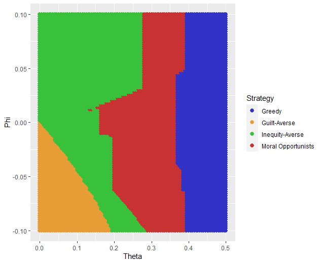
We want to plot the Free Parameters - each row as a point with the color being the groups assigned based on HAC. Let’s name our clusters based on the way we sketched out our parameter space - the three motives we identified and the behavioral strategy of Moral Opportunism we identified. The top left of the parameter space is Inequity-Aversion. The top right of the parameter space is Guilt-Aversion. The far right of the parameter space is Greed. The rest of the parameter space is the Moral Opportunism strategy.

R

freeParameters$Strategy = as.character(fit)
freeParameters$Strategy[which(freeParameters$Strategy == freeParameters$Strategy[1])] = 'Guilt-Averse'
freeParameters$Strategy[which(freeParameters$Strategy == freeParameters$Strategy[10101])] = 'Greedy'
freeParameters$Strategy[which(freeParameters$Strategy == freeParameters$Strategy[100])] = 'Inequity-Averse'
freeParameters$Strategy[which(freeParameters$Strategy != 'Inequity-Averse' & freeParameters$Strategy != 'Greedy' & freeParameters$Strategy != 'Guilt-Averse')] = 'Moral Opportunists';
freeParameters$Strategy = as.factor(freeParameters$Strategy) #Strategy clusters
model_space = ggplot(data = freeParameters, aes(x = theta, y = phi, color = Strategy)) +
labs(x = 'Theta', y = 'Phi', color = 'Strategy') + geom_point(size = 2.5) +
scale_color_manual(values = c(rgb(50,50,200, maxColorValue = 255), rgb(230,157,54, maxColorValue = 255), rgb(57,193,59, maxColorValue = 255),
                                rgb(200,50,50, maxColorValue = 255))); model_space

MatLab

Strategy = cellstr(num2str(fit));
Strategy(strcmp(Strategy, Strategy(1))) = {'Guilt-Averse'};
Strategy(strcmp(Strategy, Strategy(10101))) = {'Greedy'};
Strategy(strcmp(Strategy, Strategy(100))) = {'Inequity-Averse'};
Strategy(~ismember(Strategy, {'Inequity-Averse', 'Greedy', 'Guilt-Averse'})) = {'Moral Opportunists'};
Strategy = categorical(Strategy);

for i = 1:nrows
    for j = 1:ncols
        index = (i - 1) * ncols + j;
        freeParameters(i, j).predictions = Strategy(index);
    end
end

model_space = gca;
hold on;

for i = 1:nrows
    for j = 1:ncols
        scatter(freeParameters(i, j).theta, freeParameters(i, j).phi, 40, freeParameters(i, j).Strategy, 'filled');
    end
end
xlabel('Theta');
ylabel('Phi');
colormap([50 50 200; 230 157 54; 57 193 59; 200 50 50] / 255);
colorbar('Ticks', 1:4, 'TickLabels', {'Guilt-Averse', 'Greedy', 'Inequity-Averse', 'Moral Opportunists'});

hold off;

Python

import pandas as pd
import seaborn as sns

fit_char = fit.astype(str).tolist()

freeParameters['Strategy'] = fit_char
freeParameters.loc[freeParameters['Strategy'] == freeParameters['Strategy'][0], 'Strategy'] = 'Guilt-Averse'
freeParameters.loc[freeParameters['Strategy'] == freeParameters['Strategy'][10101], 'Strategy'] = 'Greedy'
freeParameters.loc[freeParameters['Strategy'] == freeParameters['Strategy'][100], 'Strategy'] = 'Inequity-Averse'
freeParameters.loc[~freeParameters['Strategy'].isin(['Inequity-Averse', 'Greedy', 'Guilt-Averse']), 'Strategy'] = 'Moral Opportunists'
freeParameters['Strategy'] = pd.Categorical(freeParameters['Strategy'])

model_space = sns.scatterplot(data=freeParameters, x='theta', y='phi', hue='Strategy', palette={
    'Guilt-Averse': (50/255, 50/255, 200/255),
    'Greedy': (230/255, 157/255, 54/255),
    'Inequity-Averse': (57/255, 193/255, 59/255),
    'Moral Opportunists': (200/255, 50/255, 50/255)
})
plt.xlabel('Theta')
plt.ylabel('Phi')
plt.legend(title='Strategy')
plt.show()

Examine Model Predictions Efficiently

Plain English

During this stage, you want to visualize the Decisions predicted by your model based on which cluster they fall into, visualizing the variance ideally, and considering the Independant Variables. This will allow you to gather a clearer picture of the differences predicted by your model.

R

toPlot = data.frame()
for (i in 1:length(freeParameters[,1])){
    replacement = ((i - 1) * 60 + 1):(i * 60)
    toPlot[replacement, 1] = freeParameters$Strategy[i]
    toPlot[replacement, 2] = trialList$Investment
    toPlot[replacement, 3] = trialList$Multiplier
    toPlot[replacement, 4] = as.numeric(predictions[i,])
}
colnames(toPlot) = c('Strategy', 'Investment', 'Multiplier', 'Return')

ggplot(data = toPlot[which(toPlot$Multiplier==2),], aes(x = Investment, y = Return, group = Strategy, color = Strategy)) + geom_smooth(se = TRUE) +
scale_color_manual(values = c(rgb(50,50,200, maxColorValue = 255), rgb(230,157,54, maxColorValue = 255), rgb(57,193,59, maxColorValue = 255),
                                rgb(200,50,50, maxColorValue = 255))) + lims(x = c(0, 10), y = c(0, 30))

ggplot(data = toPlot[which(toPlot$Multiplier==4),], aes(x = Investment, y = Return, group = Strategy, color = Strategy)) + geom_smooth(se = TRUE) +
scale_color_manual(values = c(rgb(50,50,200, maxColorValue = 255), rgb(230,157,54, maxColorValue = 255), rgb(57,193,59, maxColorValue = 255),
                                rgb(200,50,50, maxColorValue = 255))) + lims(x = c(0, 10), y = c(0, 30))

ggplot(data = toPlot[which(toPlot$Multiplier==6),], aes(x = Investment, y = Return, group = Strategy, color = Strategy)) + geom_smooth(se = TRUE) +
scale_color_manual(values = c(rgb(50,50,200, maxColorValue = 255), rgb(230,157,54, maxColorValue = 255), rgb(57,193,59, maxColorValue = 255),
                                rgb(200,50,50, maxColorValue = 255))) + lims(x = c(0, 10), y = c(0, 30))

MatLab

toPlot = table();
for i = 1:(ncols.*nrows)
    replacement = ((i - 1) * 60 + 1):(i * 60);
    toPlot(replacement, 1) = table(Strategy(i));
    toPlot(replacement, 2) = table(trialList.Investment);
    toPlot(replacement, 3) = table(trialList.Multiplier);
    toPlot(replacement, 4) = table(data_matrix(i,:));
end

toPlot.Properties.VariableNames = {'Strategy', 'Investment', 'Multiplier', 'Return'};

figure;
subplot(1, 3, 1);
dataSubset = toPlot(toPlot.Multiplier == 2,:);
scatter(dataSubset.Investment, dataSubset.Return, [], dataSubset.Strategy, 'filled');
colormap([50 50 200; 230 157 54; 57 193 59; 200 50 50] / 255);
xlabel('Investment');
ylabel('Return');
title('Multiplier = 2');

subplot(1, 3, 2);
dataSubset = toPlot(toPlot.Multiplier == 4,:);
scatter(dataSubset.Investment, dataSubset.Return, [], dataSubset.Strategy, 'filled');
colormap([50 50 200; 230 157 54; 57 193 59; 200 50 50] / 255);
xlabel('Investment');
ylabel('Return');
title('Multiplier = 4');

subplot(1, 3, 3);
dataSubset = toPlot(toPlot.Multiplier == 6,:);
scatter(dataSubset.Investment, dataSubset.Return, [], dataSubset.Strategy, 'filled');
colormap([50 50 200; 230 157 54; 57 193 59; 200 50 50] / 255);
xlabel('Investment');
ylabel('Return');
title('Multiplier = 6');

Python

toPlot = pd.DataFrame(columns=['Strategy', 'Investment', 'Multiplier', 'Return'])

for i in range(len(freeParameters)):
    replacement = list(range((i * 60) + 1, (i + 1) * 60 + 1))
    toPlot.loc[replacement, 'Strategy'] = freeParameters.loc[i, 'Strategy']
    toPlot.loc[replacement, 'Investment'] = trialList['Investment']
    toPlot.loc[replacement, 'Multiplier'] = trialList['Multiplier']
    toPlot.loc[replacement, 'Return'] = predictions[i, :].astype(float)

toPlot['Multiplier'] = toPlot['Multiplier'].astype(int)

plt.figure(figsize=(8, 6))
sns.lineplot(data=toPlot[toPlot['Multiplier'] == 2], x='Investment', y='Return', hue='Strategy', palette={
    'Guilt-Averse': (50/255, 50/255, 200/255),
    'Greedy': (230/255, 157/255, 54/255),
    'Inequity-Averse': (57/255, 193/255, 59/255),
    'Moral Opportunists': (200/255, 50/255, 50/255)
})
plt.xlim(0, 10)
plt.ylim(0, 30)
plt.legend(title='Strategy')
plt.show()

plt.figure(figsize=(8, 6))
sns.lineplot(data=toPlot[toPlot['Multiplier'] == 4], x='Investment', y='Return', hue='Strategy', palette={
    'Guilt-Averse': (50/255, 50/255, 200/255),
    'Greedy': (230/255, 157/255, 54/255),
    'Inequity-Averse': (57/255, 193/255, 59/255),
    'Moral Opportunists': (200/255, 50/255, 50/255)
})
plt.xlim(0, 10)
plt.ylim(0, 30)
plt.legend(title='Strategy')
plt.show()

plt.figure(figsize=(8, 6))
sns.lineplot(data=toPlot[toPlot['Multiplier'] == 6], x='Investment', y='Return', hue='Strategy', palette={
    'Guilt-Averse': (50/255, 50/255, 200/255),
    'Greedy': (230/255, 157/255, 54/255),
    'Inequity-Averse': (57/255, 193/255, 59/255),
    'Moral Opportunists': (200/255, 50/255, 50/255)
})
plt.xlim(0, 10)
plt.ylim(0, 30)
plt.legend(title='Strategy')
plt.show()

Tutorial 2 - Galvan & Sanfey, 2024

Choosing an Approach to Grouping

Our four choices are: no grouping, binning, a priori clustering, or post-hoc clustering. Since we want to study people based on the strategy that they use to make decisions and our model is not using noise parameters, let’s group. The reason we don’t have to include noise parameters is because we are offering several choices per trial, so a priori clustering is on the table. Binning isn’t appropriate here because we’re looking for 4 strategies and the cutoffs between these strategies are kind of fuzzy - we don’t want to arbitrarily assign boundaries between strategies if we can avoid it. Post-hoc clustering isn’t preferable when we can group a priori, so let’s do that.

Cluster Your Data Using HAC

R

distance_mat = dist(predictions, method = 'euclidean')
set.seed(240)
hierarchical = hclust(distance_mat, method = 'average')
plot(hierarchical)
fit = cutree(hierarchical, k = 4)

MatLab

distance_mat = pdist(predictions);
hierarchical = linkage(distance_mat, 'average');
dendrogram(hierarchical);
title('Hierarchical Clustering Dendrogram');
xlabel('Data Points');
ylabel('Distance');
fit = cluster(hierarchical, 'MaxClust', 4);

Python

from scipy.cluster.hierarchy import linkage, dendrogram, fcluster
from scipy.spatial.distance import pdist

distance_mat = pdist(predictions)
hierarchical = linkage(distance_mat, method='average')
dendrogram(hierarchical)
plt.title('Hierarchical Clustering Dendrogram')
plt.xlabel('Data Points')
plt.ylabel('Distance')
plt.show()

fit = fcluster(hierarchical, t=4, criterion='maxclust')

Identify Where Your Clusters are

R

freeParameters$Strategy = as.character(fit)
freeParameters$Strategy[which(freeParameters$Strategy == freeParameters$Strategy[1])] = 'Equity-Seeking'
freeParameters$Strategy[which(freeParameters$Strategy == freeParameters$Strategy[10101])] = 'Equality-Seeking'
freeParameters$Strategy[which(freeParameters$Strategy != 'Equity-Seeking' & freeParameters$Strategy != 'Equality-Seeking' & freeParameters$Strategy != 'Guilt-Averse')] = 'Payout-Maximizers';
freeParameters$Strategy = as.factor(freeParameters$Strategy) #Strategy clusters
model_space = ggplot(data = freeParameters, aes(x = theta, y = phi, color = Strategy)) +
    labs(x = 'Theta', y = 'Phi', color = 'Strategy') + geom_point(size = 2.5) +
    scale_color_manual(values = c(rgb(0,130,229, maxColorValue = 255), rgb(255,25,0, maxColorValue = 255), rgb(174,0,255, maxColorValue = 255))); model_space

MatLab

% Assuming fit is a variable already defined in your code
freeParameters.Strategy = cellstr(fit);

% Change values based on conditions
freeParameters.Strategy(strcmp(freeParameters.Strategy, freeParameters.Strategy{1})) = 'Equity-Seeking';
freeParameters.Strategy(strcmp(freeParameters.Strategy, freeParameters.Strategy(10101))) = 'Equality-Seeking';
freeParameters.Strategy(~ismember(freeParameters.Strategy, {'Equity-Seeking', 'Equality-Seeking', 'Guilt-Averse'})) = 'Payout-Maximizers';

% Convert to categorical
freeParameters.Strategy = categorical(freeParameters.Strategy);

% Create the scatter plot
figure;
scatter(freeParameters.theta, freeParameters.phi, 25, freeParameters.Strategy, 'filled');
xlabel('Theta');
ylabel('Phi');
title('Model Space');
colormap([0 130 229; 255 25 0; 174 0 255] / 255);
colorbar('Ticks', 1:3, 'TickLabels', {'Equity-Seeking', 'Equality-Seeking', 'Payout-Maximizers'});

Python

import pandas as pd
import numpy as np
import matplotlib.pyplot as plt

# Assuming fit is a variable already defined in your code
freeParameters['Strategy'] = fit.astype(str)

# Change values based on conditions
freeParameters.loc[freeParameters['Strategy'] == freeParameters['Strategy'][0], 'Strategy'] = 'Equity-Seeking'
freeParameters.loc[freeParameters['Strategy'] == freeParameters['Strategy'][10101], 'Strategy'] = 'Equality-Seeking'
freeParameters.loc[~freeParameters['Strategy'].isin(['Equity-Seeking', 'Equality-Seeking', 'Guilt-Averse']), 'Strategy'] = 'Payout-Maximizers'

# Convert to categorical
freeParameters['Strategy'] = pd.Categorical(freeParameters['Strategy'])

# Create the scatter plot
plt.scatter(freeParameters['theta'], freeParameters['phi'], s=25, c=freeParameters['Strategy'].cat.codes, cmap='viridis')
plt.xlabel('Theta')
plt.ylabel('Phi')
plt.title('Model Space')
plt.colorbar(ticks=[0, 1, 2], label='Strategy', ticklabels=['Equity-Seeking', 'Equality-Seeking', 'Payout-Maximizers'])
plt.show()

Examine Model Predictions Efficiently

R

toPlot = data.frame()
for (i in 1:length(freeParameters[,1])){
    replacement = ((i - 1) * 20 + 1):(i * 20)
    toPlot[replacement, 1] = freeParameters$Strategy[i]
    toPlot[replacement, 2] = as.numeric(trialList[, 1])
    toPlot[replacement, 3] = as.numeric(predictions[i, 1:20])
    toPlot[replacement, 4] = new_value(trialList[, 1], as.numeric(predictions[i, 1:20])) - trialList[, 1]
}
colnames(toPlot) = c('Strategy', 'Initial_Allocation', 'Tax_Rate', 'Payout_Change')

ggplot(data = toPlot, aes(x = Initial_Allocation, y = Payout_Change, group = Strategy, color = Strategy)) + geom_smooth(se = TRUE) +
       scale_color_manual(values = c(rgb(0,130,229, maxColorValue = 255), rgb(255,25,0, maxColorValue = 255), rgb(174,0,255, maxColorValue = 255))) +
                          lims(x = c(0, 10), y = c(0, 30)) + labs(x = 'Initial Allocation', 'Payout Change')

ggplot(data = toPlot, aes(x = Initial_Allocation, y = Tax_Rate, group = Strategy, color = Strategy)) + geom_smooth(se = TRUE) +
       scale_color_manual(values = c(rgb(0,130,229, maxColorValue = 255), rgb(255,25,0, maxColorValue = 255), rgb(174,0,255, maxColorValue = 255))) +
                          lims(x = c(0, 10), y = c(0, 30)) + labs(x = 'Initial Allocation', 'Tax Rate')

MatLab

figure;

gscatter(toPlot.Initial_Allocation, toPlot.Payout_Change, toPlot.Strategy, ...
    [rgb('0,130,229'); rgb('255,25,0'); rgb('174,0,255')], 'o', 8, 'on');
xlabel('Initial Allocation');
ylabel('Payout Change');
title('Scatter Plot with Smoothed Lines');
legend('Location', 'Best');
xlim([0, 10]);
ylim([0, 30]);
grid on;

figure;

gscatter(toPlot.Initial_Allocation, toPlot.Tax_Rate, toPlot.Strategy, ...
    [rgb('0,130,229'); rgb('255,25,0'); rgb('174,0,255')], 'o', 8, 'on');
xlabel('Initial Allocation');
ylabel('Tax Rate');
title('Scatter Plot with Smoothed Lines');
legend('Location', 'Best');
xlim([0, 10]);
ylim([0, 30]);
grid on;

Python

import seaborn as sns

plt.figure()

sns.lmplot(x='Initial_Allocation', y='Payout_Change', hue='Strategy', data=toPlot, ci='sd', palette=['#0082E5', '#FF1900', '#AE00FF'])
plt.xlabel('Initial Allocation')
plt.ylabel('Payout Change')
plt.title('Scatter Plot with Smoothed Lines')
plt.legend(loc='best')
plt.xlim(0, 10)
plt.ylim(0, 30)
plt.grid(True)

plt.figure()

sns.lmplot(x='Initial_Allocation', y='Tax_Rate', hue='Strategy', data=toPlot, ci='sd', palette=['#0082E5', '#FF1900', '#AE00FF'])
plt.xlabel('Initial Allocation')
plt.ylabel('Tax Rate')
plt.title('Scatter Plot with Smoothed Lines')
plt.legend(loc='best')
plt.xlim(0, 10)
plt.ylim(0, 30)
plt.grid(True)

plt.show()

Tutorial 3 - Crockett et al., 2014

Choosing an Approach to Grouping

Here, we have non-interesting parameters ( Beta, Epsilon, and Gamma ) which immediately rules out the possibility of a priori clustering. We could still potentially do post-hoc clustering - on both our Decisions as well as the Free Parameters we recover. However, clustering Decisions seems a less-than-optimal approach since we are expecting individual differences between Subjects in terms of how stochastic their Decisions are. Consequently, we can cluster Free Parameters - so, should we cluster Kappa and/or Lambda ?

Probably not and here’s why - our main goal is to study differences in Kappa between Conditions - namely when the shocks are administered to the Subject versus Others . If Kappa is lower in the Subject Harmed condition compared to the Other Harmed condition, they are more harm-averse for themselves than others, and vice versa. So, binning seems more appropriate for our goals here - we’ll group people based on if Kappa is lower or higher when the shocks are administered to the Subject versus Others .

Tutorial 4 - Li et al., 2022

Choosing an Approach to Grouping

Here, we have non-interesting parameters ( Beta, Epsilon, and Gamma ) which immediately rules out the possibility of a priori clustering. We don’t have Condition`s in the current design so we can’t apply the same rules-based binning approach as in the Crockett et al. study. We could look at differences between :bdg-success:`Free Parameters to determine groups (i.e. if α is bigger than δ) but we don’t have a guarantee that these are scaled in the same way necessarily. So none of these options seems particularly good.

An important thing to note is that, while grouping is often informative, we don’t need to superimpose groupings when our research question doesn’t drive them: just because we can doesn’t mean we should. We could do Post-Hoc clustering on either the Free Parameters or the Choices people make but we don’t really need to. The authors in this paper did not group and we won’t either.