Recovering Free Parameters
Lesson
Elijah Galvan
September 1, 2023
17 min read
Goal During this Stage
To estimate Free Parameters from our simulated data and to compare the recovered Free Parameters to our true Free Parameters
The Logic of Recovering Free Parameters
In essence, simulating data is a deduction - we know what the data generation process is and we know what the inputs to the data generation process are, so we deduce what data would be generated. However, participants obviously don’t walk into your laboratory with their free parameter values plastered onto their forehead so how do we get to these? The intuition of recovering free parameters is that of drawing an inference.
Here, we will illustrate this logic using our example of utility theory; we can start by reiterating the central premise of utility theory which is that people are thought to maximize their expected Utility. Therefore, we would say that, if we know an individual subject’s Decisions, we just take some random Free Parameters and calculate the Utility that they would have experienced if those were their true Free Parameter values. Obviously, we cannot make an inference with only one guess, but if we make several guesses we can identify the pair of Free Parameters which minimize the difference between observed-and-expected Utility (meaning that the person maximized their expected Utility). This pair of Free Parameters that we identify is referred to as the recovered Free Parameters. Thus, recovering Free Parameters is the process of drawing an inference - given that we know the outcome of the data generation process (Decisions) and the Experimental Variables for each trial, we can infer about the unknowns - in this case the Free Parameters which produced these Decisions.
Why Estimate Free Parameters for Simulated Data?
So now we know what we’re generally trying to achieve with computational modeling, but why are we talking about estimate Free Parameters now? After all, we haven’t collected any data at this stage - the only data we have is the data we’ve simulated and why would we want to recover Free Parameters we already know in the first place? This seems rather silly at first glance, but estimating Free Parameters from simulated data (i.e. parameter recovery) is the most important thing we will do at this stage of computational modeling. Our model obviously has made some specific predictions in terms of behavior: for each pair of Free Parameters, we have a single predicted Decision for each Trial. However, our ability to draw an inference about Free Parameters relies on the fact that Decisions predicted by the model can be reliably ‘mapped onto’ the true Free Parameters values.
If the Free Parameters we recover from the the predicted Decisions are similar enough to the Free Parameters which created the data, we can be confident that the Free Parameters we recover from subjects’ Decisions will be useful estimates of their preferences in this task.
Defining Error Between Expected Utility and Observed Utility.
So how do we recover Free Parameters from Decisions? In theory, we’ve already answered that: we’re going to take the Free Parameters which minimize the error between expected Utility and observed Utility. 2 common ways of defining this error are Maximum Likelihood Estimation and Ordinary Least Squares. Here’s are some copy-and-pasted explanations from ChatGPT which I found to be concise and helpful.
Maximum Likelihood Estimation
Maximum Likelihood Estimation (MLE) is typically used when you have a parametric statistical model and you want to estimate the parameters that maximize the likelihood of the observed data given the model.
MLE is often used in models where the error terms are assumed to follow a specific distribution, such as the normal distribution.
MLE provides estimates that are asymptotically efficient and consistent.
Note
Maximum Likelihood Estimation is a bit of a misnomer in this instance: although Likelihood is sometimes used to estimate values, here we don’t consider Likelihood but Negative Log Likelihood. Thus, for our purposes MLE refers to Minimum Negative Log Likelihood Estimation (MNLLE).
Ordinary Least Squares
Ordinary Least Squares (OLS) is commonly used for linear regression models where the goal is to minimize the sum of squared residuals between the observed data and the predicted values.
OLS assumes that the errors are normally distributed, and it provides estimates that are unbiased and have the minimum variance among linear unbiased estimators.
OLS is computationally efficient and easy to interpret.
We’re going to whichever was used in each paper for the tutorials, so the objective function that I will call will have an argument to choose between the two. MLE will be based on a normal distribution - the same assumption as is made by OLS. Predictably, the choice of MLE versus OLS has no bearing on the results in any paper.
How to Achieve this Goal
Objective Functions
Objective Functions take in arguments and provide, as an output, something that tells us about progress towards some objective. That’s a bit abstract but let’s remember what we just learned: OLS and MLE (or MNLLE as we specified) output values. Here lower error means better parameter fit. Thus, objective function would output error - progress towards the objective would consititute decreasing error. Let’s write an objective function which returns error, given observed Decisions and proposed Free Parameters
Take in the Trial Set, observed Decisions, and some proposed Free Parameters as inputs
Compute Utility for each possible Decision for each Trial
Select the highest possible Utility value for each Trial as the Expected Utility
Compute the Observed Utility for each observed Decision
Return the error between Expected Utility and Observed Utility
obj_function = function(params, df, method = "OLS") {
    Parameter1 = params[1]
    Parameter2 = params[2]

    k = length(as.vector(df[1,]) )#must define depending on where the decisions will be in your df, this assumes last column
    decisions = df[,k]
    trialList = df[,1:(k-1)]

    predicted_utility = vector('numeric', length(trialList[,1]))
    observed_utility = vector('numeric', length(trialList[,1]))
    for (k in 1:length(trialList[,1])){
        IV = trialList[k, 1]
        Constant = trialList[k, 2]
        Choices = #

        Utility = vector('numeric', length(Choices))
        for (n in 1:length(Choices)){
            Utility[n] = utility(Parameter1, Parameter2,
                                 construct1(IV, Constant, Choices[n]),
                                 construct2(IV, Constant, Choices[n]),
                                 construct3(IV, Constant, Choices[n]))
        }
        predicted_utility[k] = max(Utility)
        observed_utility[k] = Utility[k]
    }
    if (method == "OLS"){
        return(sum((predicted_utility - observed_utility)**2))
    } else if (method == "MLE"){
        return(-1 * sum(dnorm(observed_utility, mean = predicted_utility, sd = sd, log = TRUE)))
    }
}
function obj_value = obj_function(params, df, method)
    if nargin < 3
        method = 'OLS';
    end
    Parameter1 = params(1);
    Parameter2 = params(2);

    k = length(table2array(df(1,:))); % must define depending on where the decisions will be in your df, this assumes last column
    decisions = table2array(df(:, k));

    trialList = table2array(df(:, 1:(k-1)));


    predicted_utility = zeros(length(trialList), 1);
    observed_utility = zeros(length(trialList), 1);
    for k = 1:length(trialList)
        IV = trialList(k, 1);
        Constant = trialList(k, 2);
        Choices = #something;

        Utility = zeros(length(Choices), 1);
        for n = 1:length(Choices)
            Utility(n) = utility(Parameter1, Parameter2,
                                 construct1(IV, Constant, Choices(n)),
                                 construct2(IV, Constant, Choices(n)),
                                 construct3(IV, Constant, Choices(n)));
        end
        predicted_utility(k) = max(Utility);
        observed_utility(k) = Utility(chosen(k));
    end

    if strcmp(method, 'OLS')
        obj_value = sum((predicted_utility - observed_utility).^2);
    elseif strcmp(method, 'MLE')
        obj_value = -1 * sum(log(normpdf(observed_utility, predicted_utility, sd)));
    end
end
from scipy.stats import norm

def obj_function(params, df, method="OLS"):
    Parameter1 = params[0]
    Parameter2 = params[1]

    k = len(df.columns)  # must define depending on where the decisions will be in your df, this assumes last column
    decisions = df.iloc[:, -1].to_numpy()

    trialList = df.iloc[:, :-1].to_numpy()

    predicted_utility = np.zeros(len(trialList))
    observed_utility = np.zeros(len(trialList))

    for k in range(len(trialList)):
        IV = trialList[k, 0]
        Constant = trialList[k, 1]
        Choices = #something

        Utility = np.zeros(len(Choices))
        for n in range(len(Choices)):
            Utility[n] = utility(Parameter1, Parameter2, construct1(IV, Constant, Choices[n]), construct2(IV, Constant, Choices[n]), construct3(IV, Constant, Choices[n]))

        predicted_utility[k] = np.max(Utility)
        observed_utility[k] = Utility[chosen[k]]

    if method == "OLS":
        return np.sum((predicted_utility - observed_utility) ** 2)
    elif method == "MLE":
        sd = 1
        log_likelihood = np.sum(norm.logpdf(observed_utility, loc=predicted_utility, scale=sd))
        return -log_likelihood
Optimizers
Optimizers provide optimal solutions for objective functions. Thus, they take Decisions as fixed inputs and they provide optimal values for Free Parameters - optimal in the sense that they best achieve a specified objective. Here, that objective would be to either minimize or maximize the output of the Objective Function we just created. Thus, the Free Parameters supplied by our optimizer produce the predicted Decisions whose Expected Utility is least different from the Utility produced from the Observed Decisions. Importantly, we are optimizing on Utility which is psychological rather than Decisions which is behavioral - to fit on Decisions would be a logical fallacy.
Here, you will provide the Upper and Lower Boundaries for your Free Parameters if applicable, as well as the starting values for each of the Free Parameters. You will also need to preallocate vectors for your recovered free parameters.
Note
You also may wish to subset your Free Parameters, as to avoid long waiting times. Often, around the order of 100 recovered points will be more than sufficient - it is preferable to doing our full simulated data set which will take around 2-3 hours. As a rule of thumb, 10 to the number of Free Parameters (here 2) is a good resolution. Here, parameter1_true and parameter2_true each are a subset of Free Parameters.
Then, we want to loop around each pair of Free Parameters we are recovering values for and we are going to hand our optimizer the predicted Decisions for those Free Parameters. Then we want to save the Free Parameters recovered by that optimizer to parameter1_recovered and parameter2_recovered - these are the values that our optimizer thinks determined the predicted Decisions.
library(pracma)

initial_params = #something
lower_bounds = #something
upper_bounds = #something
parameter1_recovered = #something
parameter2_recovered = #something
parameter1_true = #something
parameter2_true = #something

for (i in 1:length(parameter1_true)) {
    df = trialList
    df$Decisions = as.numeric(predictions[this_idx,])
    this_idx = which(parameter1_true[i] == freeParameters$Parameter1 & parameter2_true[i] == freeParameters$Parameter2)
    result = fmincon(obj_function,x0 = initial_params, A = NULL, b = NULL, Aeq = NULL, beq = NULL,
                        lb = lower_bounds, ub = upper_bounds,
                        df = df)

    parameter1_recovered[i] = result$par[1]
    parameter2_recovered[i] = result$par[2]
}
initial_params = %something;
lower_bounds = %something;
upper_bounds = %something;
parameter1_recovered = %something;
parameter2_recovered = %something;
parameter1_true = %something;
parameter2_true = %something;

k = 1;
for i = 1:11
    this_i = ((i - 1) * 10) + 1
    for j = 1:11
        this_j = ((j - 1) * 10) + 1
        df = trialList
        df.Decisions = freeParameters(this_i,this_j).predictions
        options = optimoptions('fmincon', 'Display', 'off');
        result = fmincon(@(params) obj_function(params, df, 'OLS'), initial_params, [], [], [], [], lower_bounds, upper_bounds, [], options);

        parameter1_recovered(k) = result(1);
        parameter2_recovered(k) = result(2);
        k = k + 1;
    end
end
from scipy.optimize import minimize

initial_params = #something
lower_bounds = #something
upper_bounds = #something
parameter1_recovered = #something
parameter2_recovered = #something
parameter1_true = #something
parameter2_true = #something

for i in range(0, len(parameter1_true)):
    this_idx = np.where((freeParameters['Parameter1'] == parameter1_true[i]) & (freeParameters['Parameter2'] == parameter2_true[i]))[0]

    df = trialList
    df['Decisions'] = predictions[this_idx,]
    result = minimize(obj_function, x0=initial_params, bounds=list(zip(lower_bounds, upper_bounds)), args= df)

    parameter1_recovered[i] = result.x[0]
    parameter2_recovered[i] = result.x[1]
Verifying Free Parameter Recovery Process
You’ll want to visualize the error in predicting the true Free Parameter values. Depending on the kind of data you have you might want to do that in different ways.
One Parameter at a Time
We want to visualize what generated the data (X axis) with what we think generated the data (Y axis). If things look highly stochastic at the extremes, we’ll think about changing the limits. If things look highly stochastc at all values, we’ll need to revamp our model or Trial Set.
library(ggplot2)

big_mistake = ((parameter1_true - parameter1_recovered)/(max(parameter1_true) - min(parameter1_true))) > 0.25 #more than 25% of the largest possible error, can adjust to visualize better
qplot(x = parameter1_true, y = parameter1_recovered, color = big_mistake, geom = 'point')
big_mistake = ((parameter1_true - parameter1_recovered) / (max(parameter1_true) - min(parameter1_true))) > 0.25; % more than 25% of the largest possible error, can adjust to visualize better
scatter(parameter1_true, parameter1_recovered, 30, big_mistake, 'filled'); % scatter plot with big_mistake as color
colormap([0.8 0.8 0.8; 1 0 0]); % set color map to gray and red
colorbar('Ticks', [0 1], 'TickLabels', {'No', 'Yes'}); % show colorbar
xlabel('parameter1_true');
ylabel('parameter1_recovered');
import matplotlib.pyplot as plt

big_mistake = ((parameter1_true - parameter1_recovered) / (np.max(parameter1_true) - np.min(parameter1_true))) > 0.25  # more than 25% of the largest possible error, can adjust to visualize better

plt.scatter(parameter1_true, parameter1_recovered, c=big_mistake, cmap=plt.cm.RdYlGn, s=30, edgecolors='k')  # scatter plot with big_mistake as color
plt.colorbar(ticks=[0, 1], label='Big Mistake', orientation='vertical', pad=0.2)  # show colorbar
plt.xlabel('parameter1_true')
plt.ylabel('parameter1_recovered')
plt.show()
Two Parameters at a Time
We want to plot the magnitude of the error as a function of space. So we can use attributes like color and/or size to represent the distance between the True and Recover Free Parameter values.
library(ggplot2)

distance = sqrt((parameter1_true - parameter1_recovered)**2 + (parameter2_true - parameter2_recovered)**2) #calculate spatial distance in parameter recovery
max_distance = sqrt((max(parameter1_true) - min(parameter1_true))**2 + (max(parameter2_true) - min(parameter2_true))**2) #calculate maximum spatial distance
qplot(x = parameter1_true, y = parameter2_true, color = distance, size = distance, geom = 'point') + scale_radius(limits=c(0, max_distance), range=c(0, 20)) #0 is minimum distance
distance = sqrt((parameter1_true - parameter1_recovered).^2 + (parameter2_true - parameter2_recovered).^2); % calculate spatial distance in parameter recovery
max_distance = sqrt((max(parameter1_true) - min(parameter1_true)).^2 + (max(parameter2_true) - min(parameter2_true)).^2); % calculate maximum spatial distance
scatter(parameter1_true, parameter2_true, distance, distance, 'filled'); % scatter plot with distance as color and size
caxis([0, max_distance]); % set color axis limits
colorbar; % show colorbar
import matplotlib.pyplot as plt

distance = np.sqrt((parameter1_true - parameter1_recovered)**2 + (parameter2_true - parameter2_recovered)**2)  # calculate spatial distance in parameter recovery
max_distance = np.sqrt((np.max(parameter1_true) - np.min(parameter1_true))**2 + (np.max(parameter2_true) - np.min(parameter2_true))**2)  # calculate maximum spatial distance
plt.scatter(parameter1_true, parameter2_true, c=distance, s=distance, cmap='viridis', alpha=0.7)  # scatter plot with distance as color and size
plt.colorbar(label='Distance')  # show colorbar
plt.xlim(np.min(parameter1_true), np.max(parameter1_true))
plt.ylim(np.min(parameter2_true), np.max(parameter2_true))
plt.show()
Fixing Nonspecific Models
More than likely, we shouldn’t see anything that surprises us because we’ve reasoned through what our model should predict but for now let’s say that we have some work to do to improve our model before data collection. What that work which our model needs depends on the nature of our results - there are usually one of four things which can improve recovery:
We need to change our experimental design because we cannot to behaviorally distinguish between the psychological differences we are interested in (a logical place to start would be the task itself, our Trial distribution, and the Decision choices)
We need to restructure our equation because predictions made by the model do not currently reflect individual differences captured in our Free Parameters
We need to limit the range of our Free Parameters because the model predictions do not change and, therefore, are not specific.
We need to consider if the error computation in the model (i.e. the utility error) is suitable for our type of data: most models do and should assume Gaussian error but this may differ in some circumstances
On the other hand, if the recovered Free Parameters are unreliable only beyond a parameter value (i.e. for a Free Parameter ranging from 0 to 1, past 0.5 the Free Parameters we recover seem to be arbitrary and range from 0.5 to 1), we would determine that we should limit the range of Free Parameters for that range of values (in this example, instead of ranging from 0 to 1, the Free Parameter should only range from 0 to 0.5). Importantly, the converse would not be true - if meaningful psychological differences extended beyond the defined range of values for a Free Parameter, we would not be able to determine that we should extend the range of our Free Parameters at this stage. Thus, when in doubt, we should simulate over a broader range than might be necessary so that we can be confident that we are capturing the true data generation process, not only a small portion of it. If you fail to do this, you can still catch your mistake during data analysis, but the computational power to estimate Free Parameters for your sample will be much greater, the time and effort involved to correct this error will be much greater, and you will have deviated from your preregistration -all of which you can avoided by simply being punctual. This, again, is a theme: putting in a little extra time and effort will save you later!
Tutorials
Tutorial 1 - van Baar, Chang, & Sanfey, 2019
Objective Functions
obj_function = function(params, df, method = "OLS") {
    Theta = params[1]
    Phi = params[2]

    df$Decision = df[, 5]
    trialList = df[, 1:4]

    predicted_utility = vector('numeric', length(trialList[,1]))
    chosen = decisions + 1
    for (k in 1:length(trialList[,1])){
        I = trialList[k, 1]
        M = trialList[k, 2]
        B = trialList[k, 3]
        E = trialList[k, 4]
        Choices = seq(0, (I * M), 1)

        Utility = vector('numeric', length(Choices))
        for (n in 1:length(Choices)){
            Utility[n] = utility(Theta, Phi, guilt(I, B, Choices[n], M), inequity(I, M, Choices[n], E), payout_maximization(I, M, Choices[n]))
        }
        predicted_utility[k] = max(Utility)
        observed_utility[k] = Utility[chosen[k]]
    }
    if (method == "OLS"){
        return(sum((predicted_utility - observed_utility)**2))
    } else if (method == "MLE"){
        return(-1 * sum(dnorm(observed_utility, mean = predicted_utility, sd = sd, log = TRUE)))
    }
}
function obj_value = obj_function(params, decisions, method)
    if nargin < 3
        method = 'OLS';  % Default method is "OLS"
    end
    Theta = params(1);
    Phi = params(2);

    predicted_utility = zeros(length(trialList), 1);
    decisions = df(:, 5)
    chosen = decisions + 1;
    for k = 1:length(predicted_utility)
        I = trialList(k, 1);
        M = trialList(k, 2);
        B = trialList(k, 3);
        E = trialList(k, 4);
        Choices = 0:(I * M);

        Utility = zeros(length(Choices), 1);
        for n = 1:length(Choices)
            Utility(n) = utility(Theta, Phi, guilt(I, B, Choices(n), M), inequity(I, M, Choices(n), E), payout_maximization(I, M, Choices(n)));
        end
        predicted_utility(k) = max(Utility);
        observed_utility(k) = Utility(chosen(k));
    end

    if strcmp(method, 'OLS')
        obj_value = sum((predicted_utility - observed_utility).^2);
    elseif strcmp(method, 'MLE')
        obj_value = -1 * sum(log(normpdf(observed_utility, predicted_utility, sd)));
    end
end
from scipy.stats import norm

def obj_function(params, decisions, method="OLS"):
    Theta = params[0]
    Phi = params[1]

    decisions = df[, 4]
    trialList = df[, 0:3]

    predicted_utility = np.zeros(len(trialList))
    chosen = decisions + 1

    for k in range(len(predicted_utility)):
        I = trialList[k, 0]
        M = trialList[k, 1]
        B = trialList[k, 2]
        E = trialList[k, 3]
        Choices = np.arange(0, (I * M) + 1, 1)

        Utility = np.zeros(len(Choices))
        for n in range(len(Choices)):
            Utility[n] = utility(Theta, Phi, guilt(I, B, Choices[n], M), inequity(I, M, Choices[n], E), payout_maximization(I, M, Choices[n]))

        predicted_utility[k] = np.max(Utility)
        observed_utility[k] = Utility[chosen[k]]

    if method == "OLS":
        return np.sum((predicted_utility - observed_utility) ** 2)
    elif method == "MLE":
        sd = 1
        log_likelihood = np.sum(norm.logpdf(observed_utility, loc=predicted_utility, scale=sd))
        return -log_likelihood
Optimizers
library(pracma)

initial_params = c(0, 0)
lower_bounds = c(0, -0.1)
upper_bounds = c(0.5, 0.1)
theta_recovered = vector('numeric', 11**2)
phi_recovered = vector('numeric', 11**2)
theta_true = rep(seq(0, 0.5, 0.05), each = 11)
phi_true = rep(seq(-0.1, 0.1, 0.02), times = 11)

for (i in 1:length(theta_true)) {
    this_idx = which(round(theta_true[i] * 2, 2)/2 == round(freeParameters$theta * 2, 2)/2 & round(phi_true[i] * 5, 2)/5 == round(freeParameters$phi * 5, 2)) #R is sometimes finnicky about dealing with numbers to different decimal places
    df = trialList
    df$Decisions = as.numeric(predictions[this_idx,])
    result = fmincon(obj_function,x0 = initial_params, A = NULL, b = NULL, Aeq = NULL, beq = NULL,
                        lb = lower_bounds, ub = upper_bounds,
                        df = df)

    theta_recovered[i] = result$par[1]
    phi_recovered[i] = result$par[2]
}
initial_params = [0, 0];
lower_bounds = [0, -0.1];
upper_bounds = [0.5, 0.1];
theta_recovered = zeros(11^2);
phi_recovered = zeros(11^2);
theta_true = repelem(0:0.05:0.5, 11);
phi_true = repmat(-0.1:0.02:0.1, 1, 11);

k = 1;
for i = 1:11
    this_i = ((i - 1) * 11) + 1
    for j = 1:11
        this_j = ((j - 1) * 11) + 1
        df = trialList
        df.Decisions = freeParameters(this_i,this_j).predictions
        options = optimoptions('fmincon', 'Display', 'off');
        result = fmincon(@(params) obj_function(params, df, 'OLS'), initial_params, [], [], [], [], lower_bounds, upper_bounds, [], options);

        theta_recovered(k) = result(1);
        phi_recovered(k) = result(2);
        k = k + 1;
    end
end
from scipy.optimize import minimize

initial_params = np.array([0, 0])
lower_bounds = np.array([0, -0.1])
upper_bounds = np.array([0.5, 0.1])
theta_recovered = np.zeros(11**2)
phi_recovered = np.zeros(11**2)
theta_true = np.repeat(np.arange(0, 0.51, 0.05), 11)
phi_true = np.tile(np.arange(-0.1, 0.11, 0.02), 11)

for i in range(0, 121):
    this_idx = np.where((freeParameters['theta'] == theta_true[i]) & (freeParameters['phi'] == phi_true[i]))[0]

    df = trialList
    df['Decisions'] = predictions[this_idx,]
    result = minimize(obj_function, x0=initial_params, bounds=list(zip(lower_bounds, upper_bounds)), args=df)

    theta_recovered[i] = result.x[0]
    phi_recovered[i] = result.x[1]
Verifying Free Parameter Recovery Process
We want to see how much distance in Parameter Space that there is between the true Free Parameter values and the recovered Free Parameters. I find that with models with parameter values that are codetermined and interdependant, it is useful to visualize the accuracy (i.e. distance) of parameter estimation in one plot. Some rules of thumb to follow when calculating distance:
Normalize the distance on each axis to be between 0 and 1 so the differences are equally important for each of your Free Parameters
Keep the existing parameter value ranges on the axes so you can look into your
Plot the true Free Parameters, not the recovered Free Parameters
Visualize distance using size (adding color helps but is not necessary)
Ensure that the size of the points is always bound between 0 and the maximum distance (sqrt(number of Free Parameters)) so that size is a meaningful estimate of distance
Visualizing the difference in true-versus-recovered Free Parameters Following These Rules
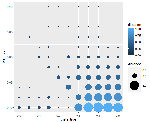
Not so great here. In the bottom right, there are some pretty big points: in fact there are 3 points which are more than 1 unit of distance away from the true value, 15 greater than 0.5 units, and 36 greater than 0.25 units. 0.25 units of distance means it’s pretty problematic - less than 5% should fit this poorly. And nothing should fit as bad to be 1 unit of distance away.
Why are we seeing what we’re seeing? Well our optimizer has a bias - it fits negative values much worse than positive values when these fits equally well which means that it would fit the positive values that badly if it had the opposite bias. More to the point, the further right we get the less meaningful the distinctions in the y-axis are.
We can clearly see why this is the case when we look at our computational model: the terms weighted by Phi are weighted by the inverse of Theta. So the predictions as Theta approach 0.5 all begin to converge on a single prediction for all values of Phi - to make Decisions that are selfish. Thus, there is still another very important rule of thumb to consider.
Remember the dependency structure between Free Parameter values as determined by the data generation process
Visualizing the difference in true-versus-recovered Free Parameters Following These Rules
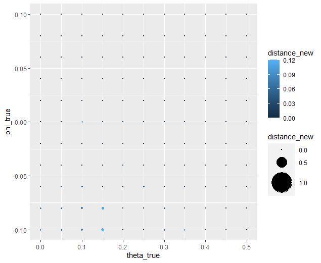
Making the distance between true and recovered Phi values decrease linearly as a function of Theta provides an theoretically and practically correct solution to our problem. Thus, we are all ready to move on since we have determined that our model makes distinct predictions and we can reliably and validly recover Free Parameters from Decisions.
library(ggplot2)

distance = (2*(theta_recovered - theta_true))**2 + (5*(phi_recovered - phi_true))**2
qplot(x = theta_true, y = phi_true, color = distance, size = distance, geom = 'point') + scale_radius(limits=c(0, sqrt(2)), range=c(0, 20))

distance_new = (2*(theta_recovered - theta_true))**2 + (5*(0.5-theta_true)*(phi_recovered - phi_true))**2
qplot(x = theta_true, y = phi_true, color = distance_new, size = distance_new, geom = 'point') + scale_radius(limits=c(0, sqrt(2)), range=c(0, 20))
distance = (2*(theta_recovered - theta_true)).^2 + (5*(phi_recovered - phi_true)).^2;
scatter(theta_true, phi_true, [], distance, 'filled');
colormap('jet');
colorbar;
xlim([0, 0.5]);
ylim([-0.1, 0.1]);
axis square;

distance_new = (2*(theta_recovered - theta_true)).^2 + (5*(0.5-theta_true).*(phi_recovered - phi_true)).^2;
scatter(theta_true, phi_true, [], distance_new, 'filled');
colormap('jet');
colorbar;
xlim([0, 0.5]);
ylim([-0.1, 0.1]);
axis square;
import matplotlib.pyplot as plt

distance = (2*(theta_recovered - theta_true))**2 + (5*(phi_recovered - phi_true))**2
plt.scatter(theta_true, phi_true, c=distance, s=distance)
plt.colorbar()
plt.xlim(0, 0.5)
plt.ylim(-0.1, 0.1)
plt.show()

distance_new = (2*(theta_recovered - theta_true))**2 + (5*(0.5-theta_true)*(phi_recovered - phi_true))**2
plt.scatter(theta_true, phi_true, c=distance_new, s=distance_new)
plt.colorbar()
plt.xlim(0, 0.5)
plt.ylim(-0.1, 0.1)
plt.show()
Tutorial 2 - Galvan & Sanfey, 2024
Objective Functions
obj_function = function(params, df, method = "OLS") {
    Theta = params[1]
    Phi = params[2]

    predicted_utility = vector('numeric', length(df[,1]))
    observed_utility = vector('numeric', length(df[,1]))
    choices = seq(0, 1, 0.1)

    for (k in 1:length(df[,1])){
        Utility = vector('numeric', length(choices))
        for (n in 1:length(choices)){
            Utility[n] = utility(theta = Theta,
                                 phi = Phi,
                                 Equity = equity(new_value(df[k, 1:10], choices[n]), df[k, 1:10], choices[n]),
                                 Equality = equality(new_value(df[k, 1:10], choices[n]), df[k, 1:10], choices[n]),
                                 Payout = payout(new_value(df[k, 1], choices[n]), df[k, 1], choices[n]))
        }
        predicted_utility[k] = max(Utility)
        observed_utility[k] = Utility[which(df[k, 11] == choices)]
    }
    if (method == "OLS"){
        return(sum((predicted_utility - observed_utility)**2))
    } else if (method == "MLE"){
        return(-1 * sum(dnorm(observed_utility, mean = predicted_utility, sd = sd, log = TRUE)))
    }
}
function obj_value = obj_function(params, df, method)
Theta = params(1);
Phi = params(2);

predicted_utility = zeros(size(df, 1), 1);
observed_utility = zeros(size(df, 1), 1);
choices = 0:0.1:1;

for k = 1:size(df, 1)
    Utility = zeros(size(choices));

    for n = 1:length(choices)
        Equity = equity(new_value(df(k, 1:10), choices(n)), df(k, 1:10), choices(n));
        Equality = equality(new_value(df(k, 1:10), choices(n)), df(k, 1:10), choices(n));
        Payout = payout(new_value(df(k, 1), choices(n)), df(k, 1), choices(n));

        Utility(n) = utility(Theta, Phi, Equity, Equality, Payout);
    end

    predicted_utility(k) = max(Utility);
    observed_utility(k) = Utility(df(k, 11) == choices);
end

if strcmp(method, 'OLS')
    obj_value = sum((predicted_utility - observed_utility).^2);
elseif strcmp(method, 'MLE')
    obj_value = -sum(log(normpdf(observed_utility, predicted_utility, sd)));
else
    error('Invalid method');
end
end
from scipy.stats import norm

def obj_function(params, df, method="OLS"):
    Theta = params[0]
    Phi = params[1]

    predicted_utility = np.zeros(len(df))
    observed_utility = np.zeros(len(df))
    choices = np.arange(0, 1.1, 0.1)

    for k in range(len(df)):
        Utility = np.zeros(len(choices))

        for n in range(len(choices)):
            Equity = equity(new_value(df[k, 0:9], choices[n]), df[k, 0:9], choices[n])
            Equality = equality(new_value(df[k, 0:9], choices[n]), df[k, 0:9], choices[n])
            Payout = payout(new_value(df[k, 0], choices[n]), df[k, 0], choices[n])

            Utility[n] = utility(Theta, Phi, Equity, Equality, Payout)

        predicted_utility[k] = max(Utility)
        observed_utility[k] = Utility[int(np.where(df[k, 10] == choices)[0])]

    if method == "OLS":
        obj_value = np.sum((predicted_utility - observed_utility)**2)
    elif method == "MLE":
        obj_value = -np.sum(np.log(norm.pdf(observed_utility, predicted_utility, sd)))
    else:
        raise ValueError("Invalid method")

    return obj_value
Optimizers
library(pracma)

initial_params = c(0.5, 0.5)
lower_bounds = c(0, 0)
upper_bounds = c(1, 1)
theta_recovered = vector('numeric', 11**2)
phi_recovered = vector('numeric', 11**2)
theta_true = rep(seq(0, 1, 0.1), length(seq(0, 1, 0.1)))
phi_true = rep(seq(0, 1, 0.1), length(seq(0, 1, 0.1)))

for (i in 1:length(theta_true)) {
    this_idx = which(round(theta_true[i], 2) == round(freeParameters$theta, 2) & round(phi_true[i], 2) == round(freeParameters$phi, 2))
    trialList_this = trialList
    trialList$Decision = as.numeric(predictions[this_idx, 1:length(trialList[1,])])
    result = fmincon(obj_function,x0 = initial_params, A = NULL, b = NULL, Aeq = NULL, beq = NULL,
                        lb = lower_bounds, ub = upper_bounds,
                        df = trialList_this)

    parameter1_recovered[i] = result$par[1]
    parameter2_recovered[i] = result$par[2]
}
addpath('path/to/pracma'); % Replace 'path/to/pracma' with the actual path to the pracma library

initial_params = [0.5, 0.5];
lower_bounds = [0, 0];
upper_bounds = [1, 1];
theta_recovered = zeros(11^2, 1);
phi_recovered = zeros(11^2, 1);
theta_true = repmat((0:0.1:1)', 1, 11);
phi_true = repelem(0:0.1:1, 11);

for i = 1:length(theta_true)
    this_idx = find(round(theta_true(i), 2) == round(freeParameters.theta, 2) & round(phi_true(i), 2) == round(freeParameters.phi, 2));
    trialList_this = trialList;
    trialList_this.Decision = predictions(this_idx, 1:length(trialList(1, :)));

    options = optimoptions('fmincon', 'Display', 'off');
    result = fmincon(@(params) obj_function(params, trialList_this), initial_params, [], [], [], [], lower_bounds, upper_bounds, [], options);

    theta_recovered(i) = result(1);
    phi_recovered(i) = result(2);
end
from scipy.optimize import minimize

initial_params = [0.5, 0.5]
lower_bounds = [0, 0]
upper_bounds = [1, 1]
theta_recovered = np.zeros(11**2)
phi_recovered = np.zeros(11**2)
theta_true = np.repeat(np.arange(0, 1.1, 0.1), 11)
phi_true = np.tile(np.arange(0, 1.1, 0.1), 11)

for i in range(len(theta_true)):
    this_idx = np.where((np.round(theta_true[i], 2) == np.round(freeParameters['theta'], 2)) & (np.round(phi_true[i], 2) == np.round(freeParameters['phi'], 2)))[0]
    trialList_this = trialList.copy()
    trialList_this['Decision'] = predictions[this_idx, :].flatten()

    result = minimize(obj_function, initial_params, args=(trialList_this,), bounds=[(0, 1), (0, 1)], method='L-BFGS-B')

    theta_recovered[i] = result.x[0]
    phi_recovered[i] = result.x[1]
Verifying Free Parameter Recovery Process
library(ggplot2)

distance = (theta_recovered - theta_true)**2 + (phi_recovered - phi_true)**2
qplot(x = theta_true, y = phi_true, color = distance, size = distance, geom = 'point') + scale_radius(limits=c(0, sqrt(2)), range=c(0, 20))

distance_new = (theta_recovered - theta_true)**2 + (((phi_recovered - 0.5) * theta_recovered) - ((phi_true - 0.5) * theta_true))**2
qplot(x = theta_true, y = phi_true, color = distance_new, size = distance_new, geom = 'point') + scale_radius(limits=c(0, sqrt(2)), range=c(0, 20))
distance = (theta_recovered - theta_true).^2 + (phi_recovered - phi_true).^2;
distance_new = (theta_recovered - theta_true).^2 + (((phi_recovered - 0.5) .* theta_recovered) - ((phi_true - 0.5) .* theta_true)).^2;

scatter(theta_true, phi_true, 20, distance, 'filled');
colormap jet;
caxis([0, sqrt(2)]);
colorbar;
xlabel('Theta True');
ylabel('Phi True');
title('Scatter Plot with Distance');

figure;

scatter(theta_true, phi_true, 20, distance_new, 'filled');
colormap jet;
caxis([0, sqrt(2)]);
colorbar;
xlabel('Theta True');
ylabel('Phi True');
title('Scatter Plot with Distance New');
import matplotlib.pyplot as plt

distance = (theta_recovered - theta_true)**2 + (phi_recovered - phi_true)**2
distance_new = (theta_recovered - theta_true)**2 + (((phi_recovered - 0.5) * theta_recovered) - ((phi_true - 0.5) * theta_true))**2

plt.scatter(theta_true, phi_true, c=distance, s=20, cmap='jet', edgecolors='none')
plt.colorbar()
plt.xlabel('Theta True')
plt.ylabel('Phi True')
plt.title('Scatter Plot with Distance')

plt.figure()

plt.scatter(theta_true, phi_true, c=distance_new, s=20, cmap='jet', edgecolors='none')
plt.colorbar()
plt.xlabel('Theta True')
plt.ylabel('Phi True')
plt.title('Scatter Plot with Distance New')

plt.show()
Tutorial 3 - Crockett et al., 2014
Objective Functions
obj_function_oneCondition = function(params, df, method = "MLE") { #we want 2 kappa parameters (1 per condition), but we don't yet have conditions
    Kappa = params[1]
    Lambda = params[2]
    Gamma = params[3]
    Epsilon = params[4]

    ProbAlternative = vector('numeric', length(df[,1]))
    for (k in 1:length(df[,1])){
        moneyDefault = c(df[k, 2], df[k, 3])[df[k, 1]]
        moneyAlternative = c(df[k, 3], df[k, 2])[df[k, 1]]
        shocksDefault = c(df[k, 4], df[k, 5])[df[k, 1]]
        shocksAlternative = c(df[k, 5], df[k, 4])[df[k, 1]]

        DiffUtility = utility(Payout = harm(shocksAlternative, shocksDefault),
                              Harm = payout(moneyAlternative, moneyDefault),
                              kappa = Kappa,
                              lambda = Lambda)
        ProbAlternative[k] = ((1)/(1 + exp(-1 * Gamma * DiffUtility))) * (1 - (2 * Epsilon)) + Epsilon
    }
    if (method == "OLS"){
        return(sum((ProbAlternative - df[, 6])**2))
    } else if (method == "MLE"){
        return(-1 * sum(dnorm(df[, 6], mean = ProbAlternative, sd = sd, log = TRUE)))
    }
}
Optimizers
library(pracma)

initial_params = c(0.5, 2, 1, 1)
lower_bounds = c(0, 1, 0, 0)
upper_bounds = c(1, 5, 10, 2)
freeParameters$kappaRecovered = 0
freeParameters$lambdaRecovered = 0
freeParameters$gammaRecovered = 0
freeParameters$epsilonRecovered = 0

for (i in 1:length(parameter1_true)) {
    result = fmincon(obj_function,x0 = initial_params, A = NULL, b = NULL, Aeq = NULL, beq = NULL,
                        lb = lower_bounds, ub = upper_bounds,
                        decisions = as.numeric(predictions[i,]))

    freeParameters$kappaRecovered[i] = result$par[1]
    freeParameters$lambdaRecovered[i] = result$par[2]
    freeParameters$gammaRecovered[i] = result$par[3]
    freeParameters$epsilonRecovered[i] = result$par[4]
}
Verifying Free Parameter Recovery Process
library(ggplot2)

#how well are we able to recover kappa and lambda?
qplot(data = freeParameters, x = kappa, y = kappaRecovered) + geom_smooth()
qplot(data = freeParameters, x = lambda, y = lambdaRecovered) + geom_smooth()

#does our inverse temperature parameter (gamma) actual capture variance in stochasticity
qplot(data = freeParameters, x = gamma, y = gammaRecovered) + geom_smooth(method = 'lm')

#is epsilon capturing loss aversion? remember, epsilon is set to 0 so it should be a nonfactor
qplot(data = freeParameters, x = lambda, y = epsilonRecovered)
Tutorial 4 - Li et al., 2022
Objective Functions
obj_function = function(params, df, optimMethod = "MLE") {
    Prob1 = generatePredictions(params, df); Chose1 = df[,7]
    if (optimMethod == "OLS"){return(sum((Chose1 - Prob1)**2))
    } else if (optimMethod == "MLE"){return(-sum(Chose1 * log(Prob1) + (1 - Chose1) * log(1 - Prob1)))}
}
Optimizers
library(pracma)

initial_params = c(1,1,1, 4, 0.25, 0)
lower_bounds = c(0, 0, 0, 0, 0, -0.5)
upper_bounds = c(2,2,2, 10, 0.5, 0.5)
freeParameters$alphaRecovered = 0
freeParameters$deltaRecovered = 0
freeParameters$rhoRecovered = 0
freeParameters$betaRecovered = 0
freeParameters$epsilonRecovered = 0
freeParameters$gammaRecovered = 0

optimize = function(obj, initial_params, lower_bounds, upper_bounds, df){
    tryCatch({
        fmincon(obj, x0 = initial_params, lb = lower_bounds, ub = upper_bounds, df = df, optimMethod = "MLE", tol = 1e-08)
    }, error = function(e){
        fmincon(obj, x0 = initial_params, lb = lower_bounds, ub = upper_bounds, df = df, optimMethod = "OLS", tol = 1e-08)
    })
}

for (i in 1:nrow(freeParameters)) {
    trialList$Predictions = as.numeric(predictions[i,])
    result = optimize(obj_function, initial_params, lower_bounds, upper_bounds, trialList)
    freeParameters$alphaRecovered[i] = result$par[1]
    freeParameters$deltaRecovered[i] = result$par[2]
    freeParameters$rhoRecovered[i] = result$par[3]
    freeParameters$betaRecovered[i] = result$par[4]
    freeParameters$epsilonRecovered[i] = result$par[5]
    freeParameters$gammaRecovered[i] = result$par[6]
    if (mod(i, round(nrow(freeParameters)/100)) == 0){message(round(100* (i/(nrow(freeParameters)))), '% there', sep = '')}
}
Verifying Free Parameter Recovery Process
library(ggplot2)

freeParameters$Epsilon = factor(freeParameters$epsilon)

qplot(data = freeParameters, x = alpha, y = alphaRecovered, color = Epsilon) + geom_smooth(se = F) + geom_abline()
qplot(data = freeParameters, x = delta, y = deltaRecovered, color = Epsilon) + geom_smooth(se = F) + geom_abline()
qplot(data = freeParameters, x = rho, y = rhoRecovered, color = Epsilon) + geom_smooth(se = F) + geom_abline()
qplot(data = freeParameters, x = beta, y = betaRecovered, color = Epsilon) + geom_smooth(se = F)+ geom_abline()
qplot(data = freeParameters, x = epsilon, y = epsilonRecovered) + geom_smooth(method = 'lm') + geom_abline()
qplot(data = freeParameters, x = gamma, y = gammaRecovered, color = Epsilon) + geom_smooth(se = F) + geom_abline()